EXAMPLE 15 Custom Waterfall Chart
Purpose: Create a waterfall chart in SAS/GRAPH, using the Annotate facility.
Waterfall charts provide a good way to visualize the cumulative effect of positive or negative data values sequentially added to a running total (such as a ledger or checkbook). A waterfall chart is similar to a line chart of the cumulative total, using the step interpolation.
As of SAS 9.2, SAS/GRAPH does not have a built-in easy way to produce waterfall charts, but as you might have guessed, you can create them fairly easily using a bit of custom programming.
Let’s start with some simple data for a small company. After reading in these values, we can calculate the total for the end of the year, and add that total as an extra observation at the end of the data set. I call this final (modified) data set MODDATA. (Note: you could hardcode the final value in your data, but I prefer to calculate values like that programmatically to guarantee they are correct.)
data bardata;
input lablvar $ 1-50 barval;
datalines;
Beginning Value 10
First Quarter -20
Second Quarter 30
Third Quarter 25
Fourth Quarter 37
End-of-Year Taxes -40
End-of-Year Kickbacks 11
;
run;
proc sql;
create table sumdata as
select 'Final Value' as lablvar, sum(barval) as barval
from bardata;
quit; run;
data moddata;
set bardata sumdata;
run;
Here is what the modified data looks like. Note that I now have an observation for the “Final Value”:
Beginning Value 10
First Quarter -20
Second Quarter 30
Third Quarter 25
Fourth Quarter 37
End-of-Year Taxes -40
End-of-Year Kickbacks 11
Final Value 53
You could produce a simple bar chart, as follows. However, with the bars in the default alphabetical order, the chart does not reflect the sequential nature of the data:
title1 ls=1.5 "Simple GChart";
axis1 label=none minor=none order=(-50 to 100 by 25) offset=(0,0);
axis2 label=none value=(angle=90);
proc gchart data=moddata;
vbar lablvar / discrete type=sum sumvar=barval
raxis=axis1 maxis=axis2
autoref cref=gray55 lref=33 clipref;
run;
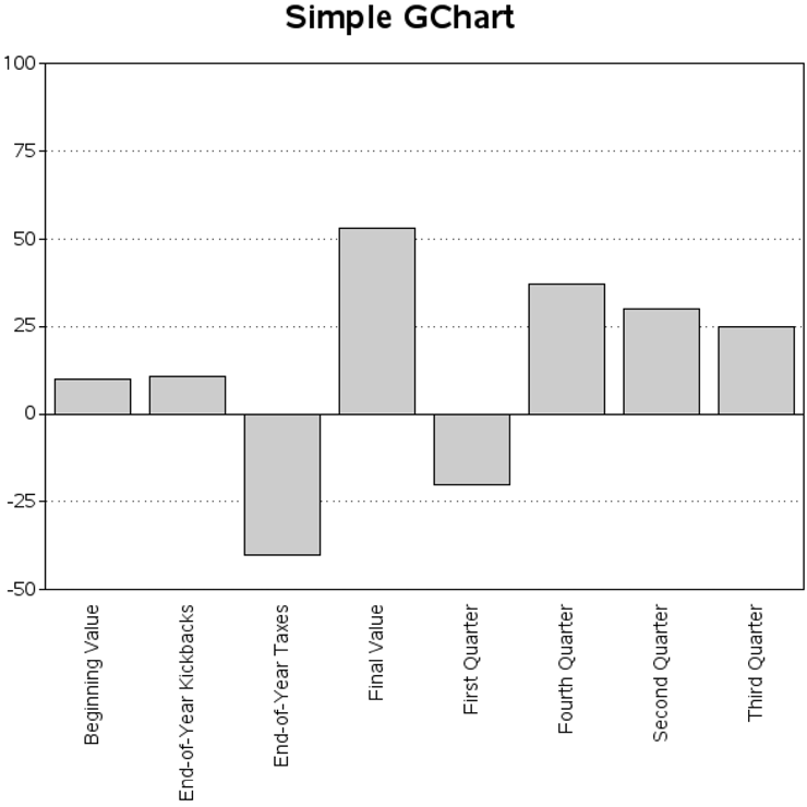
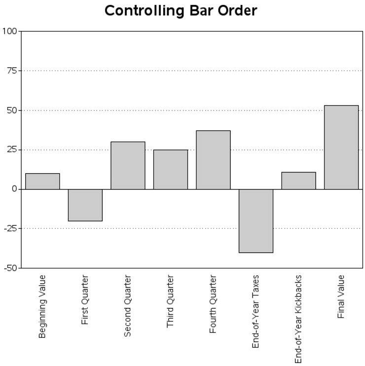
Of course you could hardcode the order of the bars in an axis statement so the bars are in the desired sequential order, as shown below. You should note, however, that hardcoding is very tedious, especially if your data changes.
axis2 label=none value=(angle=90)
order=(
'Beginning Value'
'First Quarter'
'Second Quarter'
'Third Quarter'
'Fourth Quarter'
'End-of-Year Taxes'
'End-of-Year Kickbacks'
'Final Value'
)
;
{re-run same GChart code as before}
And you could even add a variable to the data, add pattern statements, and then use PROC GCHART’s SUBGROUP= option to control the colors of the bars.
data moddata; set moddata;
if lablvar in ('Beginning Value' 'Final Value') then colorvar=1;
else if barval>=0 then colorvar=2;
else colorvar=3;
run;
pattern1 v=s c=cx499DF5; /* blue */
pattern2 v=s c=cx49E20E; /* green */
pattern3 v=s c=cxFF3030; /* red */
proc gchart data=moddata;
vbar lablvar / discrete type=sum sumvar=barval
raxis=axis1 maxis=axis2 subgroup=colorvar nolegend
autoref cref=gray55 lref=33 clipref;
run;
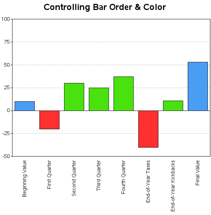
However, the result is still not a waterfall chart, and it does not tell you as much about the data as a waterfall chart could. For example, there is no indication of how each value affects the cumulative total, and therefore no indication whether the cumulative total dips below the zero line (which can be very important to know).
So let’s get busy with some custom programming.
First, let’s assign a sequential numeric value (BARNUM) to each bar, and create a user-defined format (called BAR_FMT) so those numeric values show up as the desired text values (LABLVAR). Now you can let the bars plot in their default (numeric) order, and the midpoint labels will be the text values. This technique is data-driven, eliminating the need to hardcode the text strings in the axis statement’s ORDER= option (and the need to remember to hardcode it again if the data changes). Also, the numeric values make it easier to programmatically build up the Annotate commands to “draw” the waterfall bars. The code might look a little cryptic, but you do not really have to understand how it works in order to use it. (Note that this little chunk of code is very useful and very re-usable.)
data moddata; set moddata;
barnum=_n_;
fakeval=0;
run;
data control; set moddata (rename = (barnum=start lablvar=label));
fmtname = 'bar_fmt';
type = 'N';
end = START;
run;
proc format lib=work cntlin=control;
run;
You might notice that I also assigned fakeval=0’ in the DATA step above. I use this FAKEVAL to control the bar height (sumvar=fakeval), and produce zero-height bars. This gives me a “blank slate” chart with all the bar midpoint labels and response axis but with no visible bars (since they are zero height).
proc gchart data=moddata;
format barnum bar_fmt.;
vbar barnum / discrete type=sum sumvar=fakeval
raxis=axis1 maxis=axis2 width=6
autoref cref=gray55 lref=33 clipref
nolegend noframe;
run;

The following code counts how many bars there are, so we can figure out the % width (BARWID) of each bar. The .8 value is a bit arbitrary, determined through trial-and-error, to produce visually pleasing spacing between the bars. You can adjust that value as needed.
proc sql noprint;
select count(*) into :barcount from moddata;
select (.8*(100/count(*))) into :barwid from moddata;
select (.8*(100/count(*)))/2 into :halfwid from moddata;
quit; run;
The following code uses Annotate commands to draw the bars and connect them. For positive values I draw the connecting line from the top of the bar, and for negative values I draw it from the bottom—the connecting line helps you visually “follow the money.” I use BY FAKEVAL merely as an easy way to let me test whether each observation is the first (first.fakeval) or last (last.fakeval) observation of the data set in order to handle those special cases.
Note that I add an HTML= variable to define the mouseover text and drill–down links (in Annotate, you use an HTML= variable, whereas in PROC GCHART you would use the HTML={some variable} option). To completely follow what each section of code is doing, see the detailed comments in the code.
data bar_anno; set moddata;
by fakeval;
length function $8 style $20;
when='a';
length html $500;
html=
'title='||quote( translate(trim(left(lablvar)),' ','')||
' = '||trim(left(barval)))||
' href='||quote('waterfall_anno_info.htm'),
/* If it's the first/left-most bar, start by moving to the zero line */
if first.fakeval then do;
function='move';
xsys='2'; x=barnum;
ysys='2'; y=0;
output;
end;
/* draw a horizontal line to the midpoint of the next bar */
function='draw'; color='blue';
xsys='2'; x=barnum;
ysys='7'; y=0; /* 0% up/down, from my previous y */
output;
/* Move to the left 1/2 bar width,
then draw a bar segment up/down based on the data +/- value */
function='move';
xsys='7'; x=-1*&halfwid; output;
function='bar'; color=barcolor; style='solid'; line=0;
xsys='7'; x=&barwid; /* use relative-percent coordinate system */
ysys='8'; y=barval; /* use relative-value coordinate system */
/* in the special case that it's the last bar, always connect to the zero line instead */
if last.fakeval then do;
ysys='2'; y=0;
end;
output;
run;
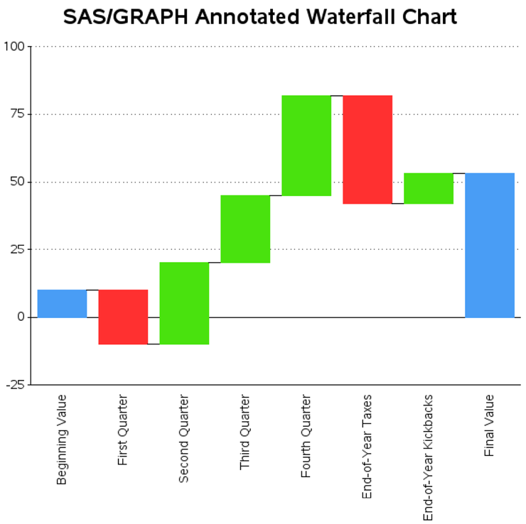
Now that we have the Annotate data set, we can run the same code we used to create the blank slate chart, but this time also specify the ANNO= option, and produce a wonderful custom waterfall chart.
title1 ls=1.5 "SAS/GRAPH Annotated Waterfall Chart";
proc gchart data=moddata anno=bar_anno;
format barnum bar_fmt.;
vbar barnum / discrete type=sum sumvar=fakeval
raxis=axis1 maxis=axis2 width=6
autoref cref=gray55 lref=33 clipref
nolegend noframe anno=anno_frame;
run;