EXAMPLE 17  Custom Calendar Chart

Purpose: The focus of this example is a little different from most of the others. While in the other examples I am mainly trying to teach you the graphical techniques so that you can modify the techniques and create your own similar but unique graphics, in this example I am mainly demonstrating how to re-use this calendar chart with your own data.

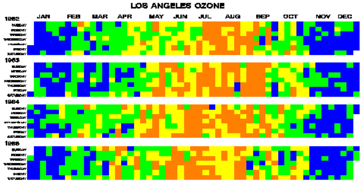
I got the idea for this graph from Michael Friendly’s Gallery of Data Visualization Web site, specifically the Bright Ideas page.1 Below is a portion of the chart, showing four of the ten years of data.

For those of you reading this online on a color display, you can see the color in this version from Friendly’s Web site:

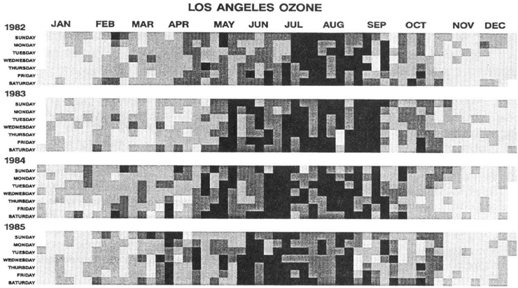
The graph also appeared in “Tracking Air Quality Trends with SAS/GRAPH,” published in the SUGI 22 proceedings.2 Here is how it appeared there, in black and white.

I thought this was a very interesting way to visualize data, and decided to write my own implementation using the SAS/GRAPH GMAP procedure.

The Response Data Set

To run this example, you will need some data similar to what appeared in the chart in the SUGI paper: a series of dates and values. I did not have access to the actual Los Angeles Ozone data. Therefore, I wrote a DATA step that loops through all the days in the chart, and generates some “plausible” random data. I recommend that you get the example running with this data first, and later substitute your own data. You can download both the data and the SAS code from the author’s Web site. 3

data my_data;

 format day date7.;

 format ozone comma5.2;

 do day = '01jan82'd to '31dec91'd by 1;

  monname=trim(left(put(day,monname.)));

  year=put(day,year.);

  ozone=ranuni(1)*.5;

  /* Simulate the ozone being better in winter months */

  if monname in ('December' 'January') then ozone=ozone/9;

  else if monname in ('November' 'February') then ozone=ozone/3.5;

  else if monname in ('September' 'October' 'March' 'April') then ozone=ozone/1.5;

  else if ozone < .15 then ozone=.15;

  /* Simulate ozone getting better in recent years */

  if year = 1991 then ozone=.9*ozone;

  if year = 1990 then ozone=.92*ozone;

  if year = 1989 then ozone=.94*ozone;

  if year = 1988 then ozone=.95*ozone;

  if year = 1987 then ozone=.96*ozone;

  if year = 1986 then ozone=.97*ozone;

  output;

 end;run;

To make it easier to explain the example and demonstrate how to handle days with “missing” data, I subset the data, demonstrate with a small subset, and then later plot the entire series.

data my_data; 

 set my_data (where=(day>='01mar1982'd and day<='15mar1982'd));

run;

Here is what the subset of data looks like. Each observation is just a date and a numeric value. In this example the numeric value is an ozone measurement, but you can actually plot anything you want, such as sales, attendance, temperature, stock price, number of patients, deaths, and so on.

  day   ozone 

01MAR82 0.02 

02MAR82 0.17

03MAR82 0.11

04MAR82 0.01

05MAR82 0.24

06MAR82 0.31

07MAR82 0.15

08MAR82 0.32

09MAR82 0.24

10MAR82 0.03

11MAR82 0.06

12MAR82 0.09

13MAR82 0.20

14MAR82 0.14

15MAR82 0.02

Now, create some macro variables based on the data values, so you will know the minimum and maximum year. While you are running PROC SQL go ahead and start your annotate data set (containing one observation for each year).

proc sql; 

select min(year) into :min_year from my_data; 

select max(year) into :max_year from my_data; 

create table my_anno as select unique year from my_data;

quit; run;

Since your data might not have observations for every single day of the calendar (for example, the fifteen days of sample data we are working with here), loop through from January 1 of the minimum year (MIN_YEAR) to December 31 of the maximum year (MAX_YEAR), and create an observation for each day. Then merge this data set with the response data so that every day is represented in the response data.

data grid_days;

 format day date7.;

 do day="01jan.&min_year"d to "31dec.&max_year"d by 1;

  weekday=put(day,weekday.);

  downame=trim(left(put(day,downame.)));

  monname=trim(left(put(day,monname.)));

  year=put(day,year.);

  output;

 end;

run;

proc sql;

 create table my_data as select * 

 from grid_days left join my_data 

 on grid_days.day eq my_data.day;

quit; run;

Now, every day has a row in the response data set, either with a data value or a SAS “missing” value.

  day   ozone 

01JAN82  .

02JAN82  .

{and so on...}

27FEB82  . 

28FEB82  . 

01MAR82 0.02 

02MAR82 0.17

03MAR82 0.11

04MAR82 0.01

05MAR82 0.24

06MAR82 0.31

07MAR82 0.15

08MAR82 0.32

09MAR82 0.24

10MAR82 0.03

11MAR82 0.06

12MAR82 0.09

13MAR82 0.20

14MAR82 0.14

15MAR82 0.02

16MAR82  .

17MAR82  .

{and so on...}

30DEC82  .

31DEC82  .

There is one optional step in preparing the response data. I highly recommend creating a variable containing the HTML tags for data tips (hover text), so your users can hover their mouse over each box (day) in the calendar and see the date and data for that day. This is very useful in helping the user become oriented and see how the days are arranged in the calendar. It also provides an easy way to investigate unusual data. Use the HTML TITLE= or ALT= tag for the data tip text, and you can also include HREF= tags to add drill-down functionality. You can name this variable anything you want (I name it MYHTMLVAR in this example). When you run PROC GMAP, you just specify this variable via the HTML= option.

data my_data; set my_data;

 length  myhtmlvar $200;

 myhtmlvar='title='|| quote( 

  put(day,downame.)||'0D'x||

  put(day,date.)||'0D'x||

  'Ozone: '||put(ozone,comma5.4)||' ppm'),

run;

The GMAP Calendar Outline

Most SAS/GRAPH programmers think of PROC GMAP as being used only to draw geographical maps. But actually, it is a quite flexible tool that can be used to draw all sorts of things.

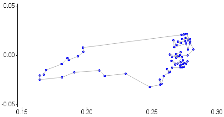
The way PROC GMAP works is that your MAP= data set contains a bunch of X and Y coordinates, and each group of coordinates forms a distinct area in the map (such as states in the US map). For example, below are the X and Y coordinates for the state of North Carolina from maps.us (plotted using a PROC GPLOT scatter plot, to demonstrate that they consist of a number of X/Y coordinates):

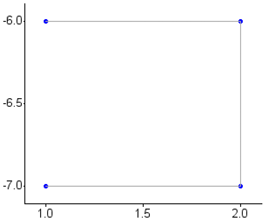
In our case, we will be creating a map where each area corresponds to a date in the calendar, with each date in the calendar being identified by 4 X and Y coordinates. Below is a PROC GPLOT scatter plot of the X and Y coordinates for January 1st, 1982:

Since calendar dates all have a predictable mathematical relationship to each other, it is a fairly simple matter to come up with the X and Y coordinates for the four corners of each date in a calendar. I use a DATA step to walk my way through all the dates, and decrement Y values (that is, go down the page) based on the year and the day of the week, and increment X values (go across the page) based on the week. Basically, the calendar days are arranged top-to-bottom, left-to-right. (Note that you must sort the data first, in order to use BY YEAR, so you can test for “first.year”.)

proc sort data=my_data out=datemap; 

by year day;

run;

data datemap; set datemap;

 keep day x y;

 by year;

 if first.year then x_corner=1;

 else if trim(left(downame)) eq 'Sunday' then x_corner+1;

 y_corner=((&min_year-year)*8.5)-weekday;

 x=x_corner; y=y_corner; output;

 x=x+1; output;

 y=y-1; output;

 x=x-1; output; 

run;

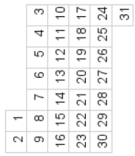
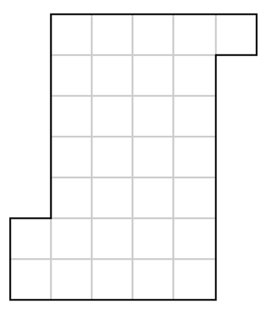
When plotted with PROC GMAP, the coordinates for January 1982 produce the following:

Here is the calendar map with the date annotated onto each box, so you can see how the days are arranged. This will help you see that it is like an actual calendar, flipped and turned on its side. As mentioned before, the days are arranged top-to-bottom left-to-right.

If you look at the original calendar plot, you will notice that it is difficult to determine where one month stops and another begins. I thought it would be useful to draw a darker outline around each month, to make the month boundaries easier to see (similar to a state outline around a county map). I do this using PROC GREMOVE and the Annotate facility, and the technique described in detail in Example 12, “Annotated Map Borders.” The resulting Annotate data set is called “Outline.”

data outline; set datemap;

length yr_mon $ 15;

yr_mon=trim(left(put(day,year.)))||'_'||trim(left(put(day,month.)));

order+1;

run;

proc sort data=outline out=outline;

by yr_mon order;

run;

proc gremove data=outline out=outline;

 by yr_mon; id day;

run;

data outline;

 length COLOR FUNCTION $ 8;

 retain first_x first_y;

 xsys='2'; ysys='2'; size=1.75; when='A'; color='black';

 set outline; by yr_mon;

 if first.yr_mon then do;

  first_x=x; first_y=y;  

  FUNCTION = 'Move'; output;

 end;

 else do;

  FUNCTION = 'Draw'; output;

 end;

 if last.yr_mon then do;

  x=first_x; y=first_y; output;

  end;

run;

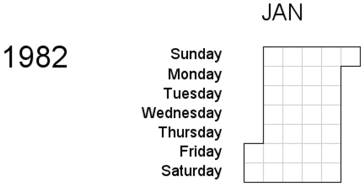
Next, I put the year and the days of the week along the left side of the chart using annotated text labels.

data my_anno; set my_anno;

length text $10;

function='LABEL';

position='4';

xsys='2'; ysys='2'; hsys='3'; when='A';

x=-8;

y=((&min_year-year)*8.5)-1.25;

style='';

size=2;

text=trim(left(year)); output;

x=-.1;

size=1;

text='Sunday'; output;

y=y-1; text='Monday'; output;

y=y-1; text='Tuesday'; output;

y=y-1; text='Wednesday'; output;

y=y-1; text='Thursday'; output;

y=y-1; text='Friday'; output;

y=y-1; text='Saturday'; output;

run;

Then, I create an Annotate data set to place the month abbreviations along the top of the page, and combine it with the MY_ANNO_DATA set. Note that I am only showing January here (so that it easily fits on the page), but the code is also creating labels for all the months.

data month_anno;

length text $10;

function='LABEL';

position='5';

xsys='2'; ysys='2'; hsys='3'; when='A';

size=1.5;

y=1;

spacing=4.5;

x=(spacing/3)*-1;

x=x+spacing; text='JAN'; output;

x=x+spacing; text='FEB'; output;

x=x+spacing; text='MAR'; output;

x=x+spacing; text='APR'; output;

x=x+spacing; text='MAY'; output;

x=x+spacing; text='JUN'; output;

x=x+spacing; text='JUL'; output;

x=x+spacing; text='AUG'; output;

x=x+spacing; text='SEP'; output;

x=x+spacing; text='OCT'; output;

x=x+spacing; text='NOV'; output;

x=x+spacing; text='DEC'; output;

run;

data my_anno; set my_anno month_anno; run;

Now here is a trick to affect the size of the resulting calendar. PROC GMAP always draws the map in the largest size possible, while still preserving the X and Y aspect ratio of the map. Therefore, depending on the proportions of your page, the calendar is quite likely to extend all the way to the left (and right) edges of the page, thereby not leaving room for the annotated text. By adding an imperceptibly small “fake” map area some distance to the left of the calendar, we can guarantee there will be room for the annotated text.

data fake;

 day=1;

 x=-11; y=1; output;

 x=x-.001; y=y+.001; output;

 x=x+.002; output;

run;

data datemap; set datemap fake;

run;

Now we plot the data. Many of the options used here are optional. Note that the XPIXELS and YPIXELS need to be specified because the calendar will not fit onto the regular default page size. ODS HTML is used so the HTML mouse-over text will work. Four pattern statements are used (in conjunction with the GMAP procedure’s levels=4) to control the colors of the days in the calendar. The DATA=, MAP=, and two ANNO= data sets point to the data sets created earlier.

%let name=calgrid;

filename odsout ".";

GOPTIONS DEVICE=png;

ODS LISTING CLOSE;

ODS HTML path=odsout body="&name..htm" 

 (title="SAS/GRAPH Custom Calendar Chart Example") style=d3d;

goptions xpixels=700 ypixels=900 border cback=white;

goptions gunit=pct htitle=4 htext=2 ftitle="albany amt/bo" ftext="albany amt";

pattern1 v=s c=cx00ff00;

pattern2 v=s c=yellow;;

pattern3 v=s c=orange;

pattern4 v=s c=red;

legend1 shape=bar(.15in,.15in) frame cshadow=gray label=none;

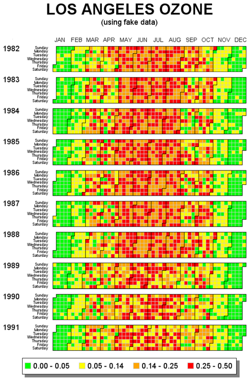
title "LOS ANGELES OZONE";

title2 "(using fake data)";

proc gmap data=my_data map=datemap all anno=my_anno; 

 id day; 

 choro ozone / levels=4 

 legend=legend1 cempty=graycc 

 coutline=graycc anno=outline 

 html=myhtmlvar name="&name"; 

run;

quit;

ODS HTML CLOSE;

ODS LISTING;

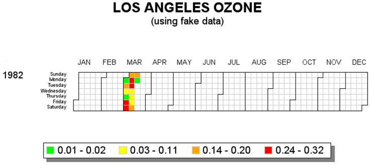
Here is what the 15 days of sample data looks like:

Using the data for all ten years (rather than just the fifteen days of March 1982), here is the final chart:

I have tried to write this example in a very generalized way, so you can easily re-use it with your own data. The only thing you should need to change is the title and the choro ozone statement.

Some final tips: If you are plotting more (or fewer) years of data, you might need to adjust the size of the page. You can do this by changing the GOPTIONS YPIXELS=, but then you will also have to change the text sizes that are scaled based on a percent of the page. These text sizes are defined in the GOPTIONS HTITLE= and HTEXT=, and also in by the SIZE= variable in the Annotate data sets. If you find yourself changing the size often, and want the annotated text to stay the same size (no matter what the YPIXELS size), then you might want to consider using hsys='D' and specifying the annotated text size in points. This is a feature added in SAS 9.2.

Also, in this example I use the simple levels=4 (quantile binning) to assign colors to the days. However, PROC GMAP supports a variety of different ways to do binning, discrete, continuous color-ramp, and so on, which you might want to learn.

Notes

1 “Tile Maps for Temporal Patterns” example from D. Mintz, T. Fitz-Simons, and M. Wayland. 1997. http://www.datavis.ca/gallery/bright-ideas.php.

2 “Tracking Air Quality Trends with SAS/GRAPH.” SUGI 22 Proceedings: 807–812. Cary, NC: SAS Institute Inc.

3 http://support.sas.com/publishing/authors/allison_robert.html.