
EXAMPLE 23 Plotting Coordinates on a Map
Purpose: Show how to plot latitude and longitude path data on a map.
As with many of my examples, this one is my imitation of an example I found on the Web. The map below originally caught my attention on Wikipedia1. I thought the map did a very good job of showing where tropical storms generally occur and what path they take. The map also graphically shows why the storms are called “tropical.”
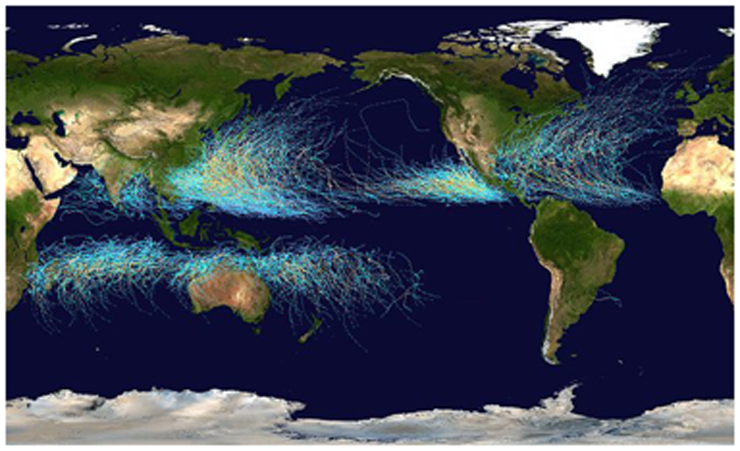
That original map is centered on the Pacific Ocean, which is a good way to map tropical storm data. However, SAS does not ship a world map arranged in that configuration. The SAS world map is centered on the Prime Meridian (LONGITUDE=0). This is why the first bit of customization is needed: in order to re-arrange the map.
I start with MAPS.WORLD from SAS, first by getting rid of the projected X and Y variables, and re-assigning the longitude and latitude to X and Y. I do this because I need X and Y to be unprojected values so that I can project them myself. While I am at it, I get rid of Antarctica (continent 97) and eliminate all the points where DENSITY is greater than 1 (so the map borders do not show too much detail).
data whole_map;
set maps.world (where=(density<=1 and cont^=97) drop=x y);
x=long;
y=lat;
run;
I plot the raw unprojected latitude and longitude points using PROC GPLOT to see what the range of X values are, and thereby determine where to split the map. PROC GPLOT is a very handy tool for easily looking at map X and Y points without having to worry about map ID variables and such.
title1 "Gplot of lat/long radians from maps.world";
symbol1 value=dot interpol=none;
proc gplot data=whole_map;
plot y*x / href=0;
run;
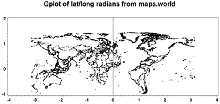
When you plot the raw X and Y points, you might notice that the land masses look backward (that is, they are a mirror image). Since this sometimes causes confusion and concern, I will try to help you understand what is going on.
When you have latitude and longitude coordinates, the longitude values start with 0 at the Prime Meridian (around London), and are usually written as the number of degrees (or radians) east or west of the Prime Meridian. For example, “80 degrees west” can be written as 80W, and “80 degrees east” as 80E. However, in a SAS data set, the longitude values are just numbers, and cannot have the “W” or “E” attached to them. Therefore, we use plus (+) and mins (–) to denote west and east, respectively. Someone had to make a decision: are values going to the west positive, or are values going to the east positive? In the case of map.world, longitude values to the west (such as the U.S.) are positive, and to the east (such as China) are denoted as negative. This is why plotting the raw (unprojected) points makes the map look backward; it is not wrong, it is just the way the data happens to be stored, and is the way PROC GPROJECT expects the X (longitude) values by default.
If you use a map where the values to the east of the Prime Meridian are positive, then you must use the EASTLONG GPROJECT option (or multiply the value by –1). The important thing to remember is that your map and Annotate X values must use the same +/– coordinate system (and sometimes you will have to multiply one or the other by –1 to make them match).
Looking at the above PROC GPLOT of the map coordinates, I determined that it would be convenient to split it at longitude value X=0. I use PROC GPROJECT with PROJECT=NONE to chop the map into two pieces. The right half contains longitude (X) values 0 to 4, and the left half contains values –4 to 0.
proc gproject data=whole_map out=right_map dupok project=none
longmin=0 longmax=4;
id id;
run;
proc gproject data=whole_map out=left_map dupok project=none
longmin=-4 longmax=0;
id id;
run;
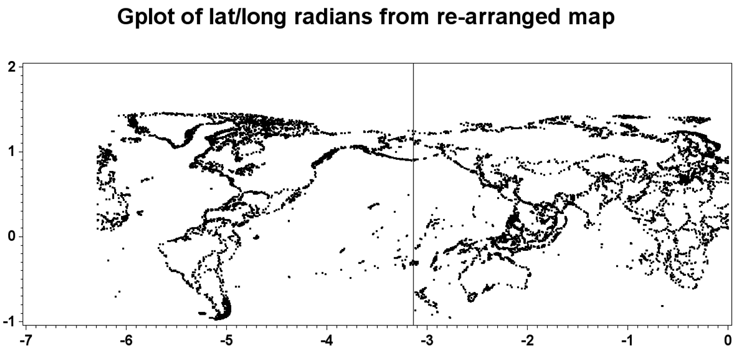
I then apply an offset to the longitude (X) values of the right side of the map, to move it to the left side (basically, I subtract 2 pi radians). And I do a little “cheat” (by adding 5000) to make sure the segments are unique. Then I put the two halves together into one data set again.
data right_map; set right_map;
segment=segment+5000;
x=x-(3.14159*2);
run;
data world_map; set right_map left_map;
run;
Here are the re-arranged X and Y points of the map, plotted with PROC GPLOT again.
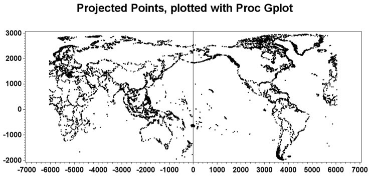
Once the latitude and longitude values are projected, the map looks correct, and we now have a world map centered on the Pacific Ocean. Here are the projected values plotted with PROC GPLOT:
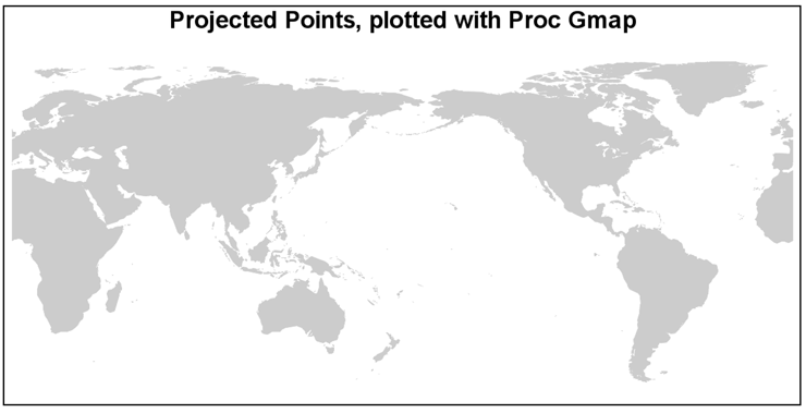
And you could now plot the map using PROC GMAP, and produce output like the following:
Now that we have the map, we need the hurricane data. After a bit of searching, I went to http://weather.unisys.com/hurricane/ and clicked on the “Best Track” link for each region. I then used the “Download Hurricane Database” link at the bottom of each region’s page.2
Reading in the data was a bit tricky, but I eventually got the data into the following format (this is just the data for one storm, to keep the example simple):
data stormdata;
input month day time lat long wind;
region='w_pacific'; year=1959; stormnum=15; snbr=324;
datalines;
9 21 18 15.8 211.5 35
9 22 0 16.2 212.4 40
9 22 6 16.6 213.3 50
9 22 12 17.1 214.2 60
9 22 18 17.5 215.1 70
9 23 0 18.2 216.1 110
9 23 6 18.8 217.1 155
9 23 12 19.5 218.0 165
9 23 18 20.2 219.0 165
9 24 0 20.8 220.0 155
9 24 6 21.6 221.0 155
9 24 12 22.4 221.9 155
9 24 18 23.4 222.8 155
9 25 0 24.4 223.6 155
9 25 6 25.6 224.3 140
9 25 12 26.8 224.3 140
9 25 18 28.3 225.1 140
9 26 0 30.1 225.1 140
9 26 6 32.2 224.7 140
9 26 12 35.3 223.4 110
9 26 18 38.3 221.1 90
9 27 0 40.6 217.8 75
9 27 6 40.2 213.5 70
9 27 12 43.0 210.0 50
9 27 18 42.2 206.0 45
9 28 0 41.5 202.0 40
9 28 6 40.8 198.0 40
9 28 12 40.0 193.0 35
;
run;
I convert the longitude and latitude from degrees to radians, and apply the same –2 pi offset to the longitude (X) of the storm data as I applied to the map. I set a flag value (ANNO_FLAG) that I will use later to identify these points as Annotate (rather than map) points. And finally, I assign a variable I can use later to keep the hurricane data points in the original (chronological) order. There is a lot going on in this little DATA step.
data stormdata; set stormdata;
x=atan(1)/45 * long;
y=atan(1)/45 * lat;
if x>0 then x=x-(3.14159*2);
anno_flag=1;
orig_order+1;
run;
Next, I combine the map and the storm data, and project the combined data set. Projecting the raw latitude and longitude coordinates enables you to control how the spherical coordinates are displayed on a flat page. There are several projection algorithms that can be used, and I chose PROJECT=CYLINDRI (cylindrical) in this example. Combining the map and the storm data and projecting them together guarantees that the projected X andY coordinates will line up properly.
data combined; set world_map stormdata; run;
proc gproject data=combined out=combined dupok norangecheck project=cylindri;
id id;
run;
After projecting the combined data set, you need to separate the map and storm data into two separate data sets, so that you will have a map data set and a storm data data set. You can do this using the ANNO_FLAG variable.
data world_map stormdata;
set combined;
if anno_flag=1 then output stormdata;
else output world_map;
run;
Now we start the process of converting the storm coordinates into an Annotate data set. First I find the maximum wind reading for each storm, and sort the storms so that the more powerful (that is, the more important) storms will be drawn last, and therefore will be more easily visible. Another alternative would be to sort the storms chronologically, so they will be drawn in that order. It all depends on what you want to emphasize in the map.
proc sql;
create table stormdata as
select unique *, max(wind) as maxwind
from stormdata
group by region, snbr;
quit; run;
proc sort data=stormdata out=stormdata;
by maxwind region snbr orig_order;
run;
Next I create a variable to uniquely identify each storm. I use the combination of region and the storm number (SNBR).
data stormdata; set stormdata;
length byvar $20;
byvar=trim(left(region))||'_'||trim(left(snbr));
run;
At the beginning of each storm (FIRST.BYVAR), I lift the Annotate pen and move to that coordinate, and for each subsequent coordinate along that storm’s path, I draw a line segment, thereby drawing the path of each storm.
data path_anno;
length function color $8 position $1;
retain xsys ysys '2' hsys '3' when 'a';
set stormdata
(keep = byvar month region snbr lat long x y wind);
by byvar notsorted;
position='5';
size=.1;
if first.byvar then do;
function='move';
output;
end;
else do;
function='draw';
color='red';
output;
end;
run;
Now that I have the Annotate data ready, all I have to do is draw a blank map (using PROC GMAP), and annotate the hurricane path (using anno=path_anno). Notice that since I am using PROC GMAP only to draw a blank map—I do not really need to specify any meaningful response data (DATA=). Therefore, I simply use the map itself as the response
data, and I specify levels=1 so that all the map areas are shaded with the color specified in PATTERN1.
pattern v=s c=graycc;
title1 height=.25in "Tracking Typhoon Vera in Year 1959";
goptions xpixels=1200 ypixels=600;
proc gmap map=world_map data=world_map anno=path_anno;
id id;
choro id / levels=1 coutline=same nolegend;
run;
And there you have it: a tropical storm path plotted in the exact right location on a world map.

In the simplified example, I hardcode the hurricane path line to be red, but in the full-fledged example (which you can download from the author’s Web page) I color-code the storms based on their wind speed.
At the top of the program, I define the colors in SAS macro variables so I can maintain them in one place and use them throughout the program.
%let colora=cx52b1ff; /* lowest */
%let colorb=cx00f8f1;
%let color1=cxffffc6;
%let color2=cxffe369;
%let color3=cxffb935;
%let color4=cxff8318;
%let color5=cxff290a; /* highest */
Then, when creating the Annotate data set, rather than using color='red', I use the following to conditionally set the color of the line:
if wind<34 then color="&colora";
else if wind<=63 then color="&colorb";
else if wind<=82 then color="&color1";
else if wind<=95 then color="&color2";
else if wind<=112 then color="&color3";
else if wind<=135 then color="&color4";
else if wind>135 then color="&color5";
else color="pink";
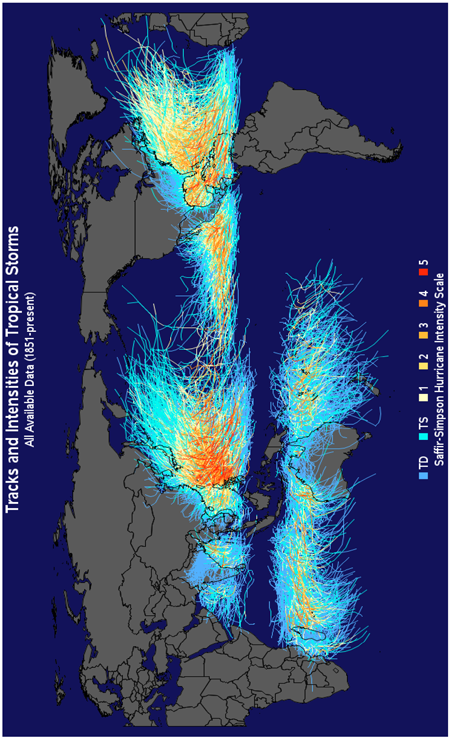
When you use the Annotate facility to create custom color graphics, you must also create your own custom legend. I sometimes use the Annotate facility to draw a legend, but in this case I use a footnote.
goptions cback=cx12125a;
pattern v=s c=cx5a5a5a;
title1 h=.25in c=white
"Tracks and Intensities of Tropical Storms";
title2 h=.18in c=white "All Available Data (1851-present)";
footnote1
f=marker h=.13in c=&colora 'U' h=.18in c=white
f="albany amt/bold" " TD "
f=marker h=.13in c=&colorb 'U' h=.18in c=white
f="albany amt/bold" " TS "
f=marker h=.13in c=&color1 'U' h=.18in c=white
f="albany amt/bold" " 1 "
f=marker h=.13in c=&color2 'U' h=.18in c=white
f="albany amt/bold" " 2 "
f=marker h=.13in c=&color3 'U' h=.18in c=white
f="albany amt/bold" " 3 "
f=marker h=.13in c=&color4 'U' h=.18in c=white
f="albany amt/bold" " 4 "
f=marker h=.13in c=&color5 'U' h=.18in c=white
f="albany amt/bold" " 5"
;
footnote2 h=.18in c=white f="albany amt/bold"
"Saffir-Simpson Hurricane Intensity Scale";
footnote3 h=.08 " ";
We use the same PROC GMAP as before, but I also specify anno=outline. This annotates the country outlines on the map (using the same technique as described in Example 12, “Annotated Map Borders”). Annotating the country outlines on top of the hurricane paths enables you to still see the country outlines, even when the country is obscured by numerous overlapping hurricanes.
proc gmap map=world_map data=world_map anno=path_anno;
id id;
choro id / levels=1 coutline=same nolegend
anno=outline;
run;
Notes
1 http://en.wikipedia.org/wiki/File:Global_tropical_cyclone_tracks-edit2.jpg .
2 Reproduced with permission of Unisys Corporation © 2011.