
Coal sampling
Abstract:
Coal sampling is fundamentally important to exploration, production and utilisation of coal. All testing and analysis results are derived from samples. This chapter gives an overview of the scientific basis of sampling based on two key characteristics of coal; particle size and particle density. The application of sampling theory to sampling systems and practical situations is discussed.
5.1 Introduction
All testing and analysis results that define the quality characteristics of a consignment of coal are obtained from a sample. The consignment could be a 60 000 tonne shipment, a day’s production, a 10 000 tonne train load, a 100 000 tonne stockpile, or any other quantity of interest. Sampling is an unavoidable feature of the coal industry, and the amount of money involved in the business of mining, processing, selling and using coal, all of which rely on analytical results, mandates that sampling is conducted using agreed scientific principles.
Sampling of coal, for the purpose of this discussion, is the extraction of a quantity of coal from a larger quantity to provide material for testing and analysis, so that the properties and composition of the larger quantity can be reliably estimated.
Differences will occur between the results from analysing samples and the true value for the quantity of coal that was sampled. These differences between the true value and the analysis results are defined as errors, and they occur because of variability in the processes and equipment used in sampling, sample preparation and analysis. The errors introduced by each of these steps is additive. That is, the total error associated with an analytical result is the sum of the errors from sampling, sample preparation and analysis. There are two fundamental types of error, systematic and random. From a sampling perspective, systematic error: relates to how the sample is collected, including the design of sampling equipment, and random error relates to the variability of the coal being sampled as well as variability in the operation of the sampling process.
Knowledge of the level of error is important, since it determines the level of confidence that can be assigned to a particular result or reported coal quality parameter, and therefore will influence decisions based on the analysis. Since sampling is potentially the source of most of the errors in coal analysis and is the first step in determining the properties of a consignment of coal, sampling operations require technical rigour in planning and execution to reduce systematic error and minimise the effects of random variations.
A large part of the error from sampling can be attributed to the number and complexity of the constituents found in coal, and understanding the complexity is fundamental to designing appropriate sampling protocols and systems. At all levels of observation, coal is made up of a diverse range of components. It is a heterogeneous material. Without taking this characteristic into account, the potential for introducing unacceptable levels of error during sampling is high. However, by understanding the heterogeneity of a coal, sampling practices can be designed to keep errors at acceptable levels. Also, by understanding the sampling characteristics of a particular coal, along with the level of precision required for analytical and test data, the most cost-effective sampling programme can be engineered. For example:
Product sampling to determine ash levels at a coal preparation plant, where the results are used to help manage plant operations, may require a sampling precision of ± 0.5% ash. On the other hand, sampling conducted at a port during ship loading of the same coal, but where the analytical results obtained from the sample form the basis of payment for the shipment, may require precision of ± 0.2% for ash. The coal preparation plant would require a significantly lower cost sampling system than that required at the port.
This chapter serves to introduce the reader to coal sampling. Much of the theory of sampling has been developed by Gy,1 who has published many works on the subject over a period of about 40 years. Lyman2,3 and Pitard4 have developed and adapted Gy’s work for its application to coal and minerals.
For a greater depth of understanding the reader is also referred to what is probably the most famous work on modern sampling known as ‘theory of sampling’ as developed by Gy; Pitard and Lyman6 have further developed and adapted the theory, especially to coal. Understanding and quantifying heterogeneity forms the basis of the sampling theory.
Other resources include the various published standard methods, such as ISO, ASTM and AS standards for coal sampling.
5.1.1 Definitions
The following definitions have been adapted from definitions given in the sampling standards.
Accuracy. A measure of the closeness of agreement between an analytical result and the true value or a reference value.
Cut. An increment taken by a sampling device or sample divider such as a sample cutter, riffle or rotary sample divider.
Bias. Systematic error which leads to the average value of a series of analytical results being persistently higher or lower than the true value or a reference sample result.
Error. Difference between the measured value and the true value or a value from a reference sample result.
Increment. An amount of coal taken from a body of coal (a truck or barge, etc.) or from a stream of coal (coal on a conveyor, sizing screen or a chute, etc.) in a single operation of the sampling device.9
Lot. Defined quantity of coal for which the quality is to be determined.
Particle top size. The nominal top size, and the square aperture size of the smallest sieve through which 95% of the sample passes.
Precision. A statistical term that quantifies how closely repeated experimental values agree. It usually has the value of the 95% confidence level, or 2 standard deviations from the mean of the experimental values.
Sample. Quantity of coal representative of a larger mass (lot) for which the quality is to be determined.
Standard deviation. A measure of the dispersion of a statistical sample, based on the square root of the mean squared deviation from the arithmetic mean.
Sublot. A part of a lot that is sampled and tested separately to the entire lot.
Tolerance. The maximum difference between measurement values or analytical results.
Variance. A measure of the spread of results expressed as the square of the standard deviation.
5.2 Accounting for heterogeneity in coal sampling
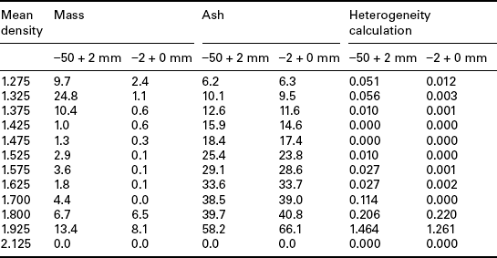
Heterogeneity pertains to the diversity of the nature of parts that make up a material. One of the most obvious aspects of the heterogeneity in coal is the range of particle sizes in a lot. Particles can be divided into size fractions, for example − 40 + 32 mm, –32 + 16 mm and so on. The mass proportion of coal in each size fraction describes the particle size distribution. In addition to size, and further adding to the heterogeneity, particles in each size fraction can be divided into density fractions which, for coal, are routinely done as part of washability testing. For example, density fractions may include sinks 1.50 floats 1.60, sinks 1.60 floats 1.70, and so on. The mass proportion of coal in each density fraction for each size fraction describes the density distribution. The particles can also have a diverse range of compositions, for example, sulphur, vitrinite, mineral matter and phosphorus. Table 5.1 shows the washability of a coal and includes the ash value as the analyte of interest for each fraction.
Table 5.1
Washability data demonstrating heterogeneity (The mass % for each density is the proportion of the total sample mass.)

At the microscopic level (Fig. 5.1) coal can be seen to be made up of different organic components or macerals derived from the original plant material, adventitious mineral matter and intrinsic mineral matter. While there is usually a strong correlation between ash% and density (higher density particles produce a higher ash% value) the species in the mineral matter that forms the ash are not likely to be uniformly distributed across size and density fractions. In addition to the solid phases, water is present and is an important parameter that requires measurement. The picture of coal becomes quite complex. Sampling needs to take into account these complexities.
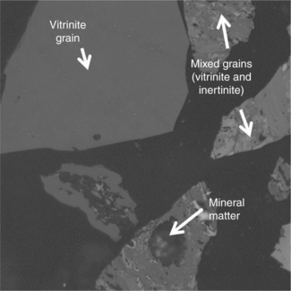
5.1 Photomicrograph of petrographic samples depicting the variable nature of the composition of coal particles at the microscopic level.
Theoretical assessment of variance attributed to the variability of coal considers heterogeneity in two forms: intrinsic heterogeneity (IH) and distributional heterogeneity (DH). IH is the average mix of the constituents within the coal, for example particles of different size and different analyte concentrations (e.g. ash%). DH occurs when the coal lot is not well mixed and the variance of a set of analyte measurements, taken at different points throughout the coal lot, is more than the variance expected from a well-mixed lot. That is, the variance is more than that attributable to IH alone. The following summary of the statistical treatment of heterogeneity and sampling demonstrates the ‘science’ behind sampling as developed by Gy. The summary serves to reinforce the requirement that sampling programmes need to have technical rigour in design and execution; otherwise the ‘garbage in garbage out’ principle will apply and there could be serious commercial and/or operational consequences for the users of the analytical data. A number of key conclusions derived from the theory are presented that are fundamental to the design, operation and analysis of sampling systems and programmes.
The theory of sampling was developed by Pierre Gy over a period of about 40 years from the 1950s. It is largely based on probability and statistics as related to the Poisson distribution and Poisson sampling. Others have also contributed to the development and application of sampling theory. In particular, Geoff Lyman has produced several papers based on Gy’s theory, some of which deal with sampling coal. It is mostly Lyman’s work on which this summary is based. For an in-depth treatment of the theory of sampling, the reader is referred to the numerous works by Gy, Lyman and others on the subject.
5.2.1 Intrinsic heterogeneity
Statistical techniques can be used to quantify IH and its contribution to the level of error in the measurement of the concentration of an analyte of interest.
Take the situation of coal on a conveyor belt. If the coal particles are divided into a range of size fractions, and each size fraction is further divided into density fractions, then the number of particles in the ith size fraction and jth density fraction can be designated as Nij, and since the length of the belt is known, the average number of particles in each size and density fraction found per unit length of the conveyor is given by Equation [5.1].
Assuming that the coal is well mixed on the belt, any increment of cross-section length ΔL of coal on the belt would be expected to yield λij = Nij/ΔL particles per increment. However, even though the coal is well mixed, there will be some random variation around this expected value.
A Poisson probability is used to describe the probability of an event or observation happening in a unit of time or length. For example,
• the number of red cars that pass a point on a highway in a day,
• the number of plant stoppages due to equipment breakdown in a week,
• the number of customers entering a fast food store every 5 min,
• the number of particles smaller than 50 mm and larger than 16 mm that float at 1.4 RD and sink at 1.5 RD that are found in every tonne of coal on a product belt from a coal preparation plant.
As the expected or mean number of observations increases, the shape of the Poisson distribution approaches that of a normal Gaussian distribution with mean μ = λ and variance σ2 = λ, as is the case for λ = 15 in Fig. 5.2.
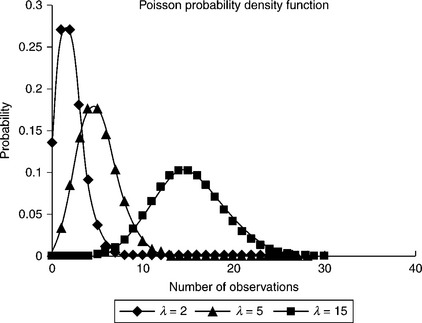
For the coal example given above, where the expected or mean number of particles per increment of cross-sectional length ΔL is concerned, the mean is μ = λij/ΔL and variance σ2 = λij/ΔL for particles in size fraction i and density fraction j. Therefore, the variance of the number of particles can be quantified, which in turn can be related to the variance in analytical results relating to each increment.
Lyman shows in Equation [5.2] the variance of analyte content ash% (As) for increments of nominal mass Ms from a well-mixed quantity of coal.
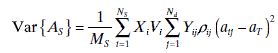
Xi = mass fraction of sample in ith class
Vi = Volume of average particle in the ith size
Yij = Mass fraction of the jth class in ith size
ρij = Density of average particle in the jth class in ith size
aij = average concentration of analyte in jth class and ith size
aT = Total concentration of the analyte in the coal
Nd = number of composition classes, or in the case of washability data, number of densities. Note that the number of densities is also the number of ash% classes.
The equation demonstrates the importance of sample mass and particle top size with respect to sampling variance.
If all parameters other than increment mass are taken as being constant i.e.
then Equation [5.2] is reduced to:
From Equation [5.3] it is obvious that in order to reduce the sampling variance the mass of the sample needs to be increased. For example, to reduce variance by a half, the mass of the increments needs to be doubled.
The volume component of the equation Vi is related to particle size and therefore variance is proportional to the cube of particle top size. If particle top size is doubled the mass of increment required to maintain the same variance is increased by 23 or 8 times. The equation clearly shows the dependence of sample or increment mass and the top size of the coal on the sampling variance.
5.2.2 Sampling constant
Further work with Equation [5.3] develops a sampling constant, Ks. Where
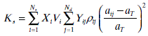
Using Ks, the sampling variance due to IH is given by
Since the parameters of Ks are density fractions ρij, the mass of the sample found in each density fraction Xi, the analyte concentration of each density fraction aij, the total analyte concentration aT, and particle volume Vi, it is possible to calculate the sampling constant Ks using washability data for coal – see Table 5.2. (Note: the volume V can be estimated for coal by multiplying the cube of the mean particle size by a shape factor, in this case 0.95.)
Table 5.2
Calculation of heterogeneity factor, precision and increment mass based on a raw coal washability
Application of the equation for variance to washability data can be used to determine the mass required to achieve a specified level of precision with respect to total ash%, as demonstrated in Table 5.2.
The consequences of what Equation [5.4] is describing include:
• For larger particle sizes, larger masses are required in order to achieve target variance values.
• Raw coals have higher Ks values and therefore more mass is required to achieve the same variance value for sampling clean coal.
• For sampling around separators in a coal preparation plant, such as a dense medium cyclone to measure the efficiency of separation, the sample of feed will need to have a higher mass than the samples of product and reject streams. The precision of the efficiency result may be adversely affected if a low mass of feed sample is collected and the variance of the feed sampling is significantly higher than the variance from the reject and product sampling. At the very least the variance of all three samples (feed, product and reject) need to be taken into account.
• Subdivision of samples in order to produce an analytical sample where only 1 or 2 g are analysed will require reduction of top size by crushing before extracting a subsample. There may be a number of top size reduction and subdivision stages required in order to produce a sample for the lab.
5.2.3 Equiprobable sampling
Given the heterogeneity of coal it follows that for a sample to be reliable and representative of the coal lot, the sampling process must be conducted so that the relative proportions of the number of particles in each size and density class are the same in the sample as they are in the coal lot from which the sample was extracted. Gy calls this ‘equiprobable sampling’. Practically it means that efforts need to be made to ensure that no size or density class of particles is preferentially favoured or disfavoured in the sampling process. For example, if a bucket used for extracting samples from a falling stream is, say, 100 mm wide and it is used in extracting increments from a coal lot with a top size of 200 mm, then obviously every coal particle greater than 100 mm has a zero chance of being included in the sample. The sample in this case cannot be representative of the coal lot, and therefore is a ‘specimen’ rather than a ‘sample’.
5.2.4 Distributional heterogeneity
DH refers to the situation where the coal properties change over time or from place to place in a body of coal such as a stockpile, rail wagon or over a day’s production from a coal preparation plant. Figure 5.3 shows the time variation of ash% for a raw coal being received at a coal preparation plant. The ash% has been determined on successive two-hourly samples. All the coal received was from a single coal seam.
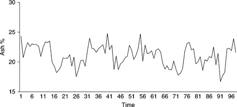
The variation in ash% over time could be a result of different sections of the seam being mined at different times and variations within the seam itself. Other causes of DH could be reclamation of coal from a segregated stockpile (e.g. where coarse coal has segregated to the base), changes in process settings in the coal preparation plant and changes in seams being mined. Figure 5.4 shows three possibilities: cyclic and continuous variation, short-term random, and long-range non-random.
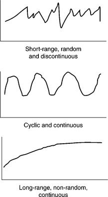
Short-term random is expected to occur in most situations when moving coal from a seam or stockpile, when unloading a ship or train, or simply as a product coal exits the coal processing plant.
Cyclic and continuous is observed on longwall operations when the top and bottom parts of the seam are mined in separate consecutive passes. It may also occur in other situations such as some stockpile reclamation operations.
Long-range non-random variation is typically found when mining starts in one part of a block of coal in a seam and progressively mines through the whole bock. For example, a longwall block starting at the eastern end works through the block over time to the western end. If the average ash increases from east to west through the block it will show as a long-range non-random increase in ash value in the raw coal over the period of mining.
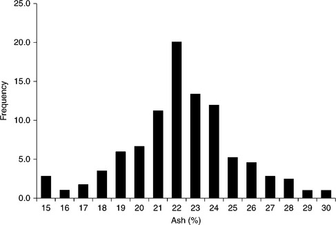
The data used in Fig. 5.3 can be presented in a distribution frequency diagram, Fig. 5.5. Lyman describes the statistics around this type of distribution, a ‘stationary discrete Gaussian random function’ and combines the variance from both intrinsic and DH in the one equation.
AS = Analyte of interest, e.g. ash%,
IH, DH refers to intrinsic and distributional heterogeneity, respectively,
aT = mean analyte concentration,
VDh = Variance resulting from distributional or long-term heterogeneity,
Equation [5.6] represents the combination of the equations for variance arising from IH and DH.
The DH variance component is the difference between total variance and variance originating from IH.
The two terms can be determined experimentally. For example, with ash% as the analyte of interest, washability data estimates the sampling constant for IH. Analysis of individual increments from a sampling scheme is used to determine the mean and variance of analyte content for DH.
5.2.5 Segregation and grouping
The variation in heterogeneity observed in coal in a stockpile, from place to place in a rail wagon, on a conveyor belt or in a feed hopper may be the result of poor mixing or segregation effects and grouping. This may be viewed as DH, but is on a relatively smaller scale. When designing a sampling system including sample preparation protocols, the possibility of segregation and/or grouping needs to be considered so that action can be taken to ensure that the sampling process is based on the equiprobable concept described earlier.
5.3 Other principles of sampling
In order to satisfy the needs of stakeholders who rely on laboratory results produced from analyzing coal samples, there are a number of other important considerations to be made. These include understanding precision and accuracy requirements, as well as the use of sampling schemes that are appropriate for the coal being sampled.
5.3.1 Precision
In coal analysis the level of precision required is usually twice the standard deviation of the sample estimate for a population. In terms of variance this becomes Equation [5.7]
where Vspt is the variance from sampling, preparation and testing and is given by Equation [5.8].
where n = the number of primary increments, VInc.
Given the relationship between precision and variance (Equation [5.8]), precision would need to be recalculated for any change in variance resulting from a change in increment mass or particle top size.
Equation [5.8] also clearly demonstrates the dependence of the magnitude of variance and therefore sampling precision, on increment mass and number of increments collected.
Variance of primary increments is a function of the variability of the coal and the method of taking the increments. Variability of coal is in turn a function of the heterogeneity of the coal and, as demonstrated, there is a strong relationship between variance and increment mass and particle top size. Variance of a measured coal property is directly related to the precision of the measured result, which in turn is an indicator of the reliability of the result and how much confidence there is that the result is indicative of the real value. Another consideration is that if a coal consignment is resampled, such as may happen when a cargo is discharged from a ship at the destination port, then the analytical results would be expected to be in agreement with those produced when the coal was sampled as the ship was loaded. However, because of variance, the results are unlikely to be exactly the same. If the results fall within the range of each other’s precision, then from a sampling and statistical perspective, they are the same. By understanding the nature of variance as applied to coal sampling, testing and analysis, differences in analytical results from separate sampling programmes on the same lot of coal can be better understood.
When determining the number of increments it is usual that the overall standard deviation of sampling, sample preparation and testing will be specified, and the primary increment standard deviation along with sample preparation and testing standard deviation will be at nominal or predetermined levels and constant. The following equation from AS 4264.1 applies.
n = number of primary increments,
σ1 = primary increment standard deviation,
σSPM = overall standard deviation of sampling, preparation and measurement,
σPM = overall standard deviation of preparation and measurement.
Since analytical results for coal testing and analysis will normally have a specified precision, β based on twice the standard deviation of the sample estimate for a population, the above equation becomes:
So assuming sampling is being conducted to determine the ash% of a coal lot with a precision of ± 0.5% and the primary increment and preparation and testing standard deviations are given as 3.0% and 0.2% respectively, the number of increments needed would be:
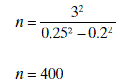
Therefore the number of increments required is 400.
If the overall precision required is ± 0.4% ash, then the number of increments would be infinite.
This problem of very large numbers of increments being required for a given level of precision may be overcome by dividing the lot of coal into a number of sublots(ns) and analysing the increments from each sublot separately followed by averaging the results over all sublots to achieve the analysis for the entire lot. The number of primary increments required is reduced significantly to yield the same specified precision. Equation [5.10] then becomes Equation [5.11] to enable the calculation of the number of increments required from each sublot. The total number of primary increments is by n × ns.
Figure 5.6 shows the change in precision of ash% determination with the number of primary increments taken for a particular coal with a primary increment variance of 3.0% and a preparation and testing variance of 0.2%. There are four plots showing the relationship for one, two, three and ten sublots. Clearly, as the number of sublots increases, the precision becomes smaller so that either a better precision is achieved or a smaller number of primary increments are required to achieve a specified level of precision. Also, from the curves it can be seen that after about 30 increments are taken, the rate of improvement in precision with increasing numbers of increments diminishes rapidly.

5.6 Use of sublots to achieve reduction in the number of primary increments for specific levels of ash % precision.
Precision and accuracy
There is often confusion between the terms precision, or precise, and accuracy. Accuracy is a measure of the closeness of agreement between an analytical result and the true value or a reference value, while precision is a measure of the spread of results or measurements. Figure 5.7 gives an example of four possible conditions where a bull’s eye target is used to present results of repeated experiments. The bull’s eye represents the true value or the reference value.

1. Precise and inaccurate, where the results are very close together but not centred on the bull’s eye of the target. For coal analysis, this occurs when the results of repeated analysis of the same sample are within a specified repeatability interval or specified tolerance, for example, ash values within ± 0.1% of each other; but the average of the values is not equal to (or within the repeatability interval around) the true value or a reference value. That is, the standard deviation of the results is small but the mean of the results is biased with respect to the true value.
2. Imprecise and inaccurate, where the results are not close together and are not centred on the bull’s eye. The coal example here is when values of repeated analysis are well outside the repeatability interval, and the mean of the values is not equal to (or within the repeatability interval around) the true value or a reference value. That is, the mean of the results is biased with respect to the true value, and the standard deviation is large.
3. Imprecise and accurate, where results are spread out and centred on the bull’s eye. For the coal ash example, the spread of repeat analysis is well outside the repeatability intervals of the ash test, but the mean is equal to or within the repeatability limit around the true or reference value. In this case the standard deviation is large and there is negligible bias of the mean of the results with respect to the true value.
4. Precise and accurate, which is the situation where results are close together and centred on the bull’s eye. Repeated ash analysis yields a spread of results that is within the repeatability interval and the mean is equal to or within the repeatability limit around the true or reference value. That is, the standard deviation of the results is small and there is negligible bias of the mean with respect to the true value.
5.3.2 Sampling schemes
Generally, primary increments can be taken at regular time or mass intervals. For time basis sampling, increments are extracted at regular time intervals. For mass basis sampling, the increments are taken at regular fixed mass intervals. The magnitude of the intervals depends on the amount of coal to be sampled and the number of increments to be extracted. In mass basis sampling the mass interval is simply determined by dividing the total mass of coal in the lot or sublot to be sampled by the number of increments that are planned to be taken. For example, it may be determined that an increment is required every 90 tonnes. Mechanical samplers would be programmed to activate the primary cutter based output from a weightometer measuring the main coal flow, or it may be assumed that there is a known constant coal flow rate and therefore the primary cutter is activated on a time basis. For example, at a flow rate of 5000 tph and an increment being required every 90 tonnes, the primary cutter is activated every 1.1 min. This type of sampling scheme is a form of a stratified sampling, and is defined as systematic sampling in AS and ISO standards.
In situations where the distributional variance may be demonstrating a cyclical behaviour, there is a risk that the simple stratified sampling scheme frequency may correlate with the variance cycle period and produce biased results. In such cases a modification to the scheme is required. A random point within each time or mass interval is selected, with the aid of a random number generator to take the primary increment. This type of scheme is referred to by ISO and AS standards as stratified random sampling. ASTM6 also acknowledges the different schemes but refers to them as ‘systematic spacing’ and ‘random spacing’.
5.3.3 Variogram
There are alternative tools that can be used to determine sampling variance. The methods based on the statistical methods discussed in this chapter do not account for autocorrelation between increments and are conservative with respect to the number of increments and sample masses required to achieve specified sampling precision levels. The variogram method determines the sampling variance and can be used to determine the number of increments required to give a specified sampling standard deviation. The method has been applied to sampling particulate materials by Gy1 and is described in AS4264.17 as well as ISO 13909–7.5
To produce a variogram for coal, increments are taken on a time- or mass-based frequency using sampling practices that conform to the appropriate standards and principles of sampling as discussed in this chapter. Each increment is analysed separately and variogram points calculated (Equation [5.12]) for the series of increments. The variogram is a plot of the mean square difference between the analyte results of two increments as a function of the number of intervals (lags) between the increments. The variogram point for a lag of 1 means that variance of analysis values from increments that are immediately adjacent to each other are used to calculate the point. For a lag of 10, the variance of analysis results for increments that are ten intervals apart are used. For time-based sampling the interval is the length of time between increments. For mass-based sampling the interval is given by the number of tonnes separating successive increments. As the interval between the increments increases the variance can be expected to increase up to a point before becoming relatively constant. However, different patterns may emerge; for example, the variogram may exhibit periodic behaviour indicating a characteristic of the coal flow that may need to be considered when designing the sampling parameters. For cyclic behaviour that cannot be corrected through process changes or relocation of sampling points, a random stratified sampling plan may yield more acceptable results for the ongoing sampling operation.
In practice, increments are taken at a regular frequency, such as every 5 min, if time-based sampling, or every 4 tonnes if massed-based sampling is employed. The variance usually becomes constant within the first ten lags. The number of increments required is specified in the Australian Standard as no less than 30. It is not specified in the ISO Standard, although the worked example given in the standard is based on 30 increments.
Variogram calculations
The value of the variogram at each lag can be calculated using the following equation.
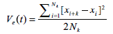
Ve(t) is the value of the variogram at lag k
ai + k is the analysis for increment i + k
ai is the analysis for increment i
Nk is the number of pairs of increments at lag k apart
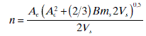
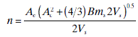
In the variogram, prior to the variance becoming constant, the increase in variance can be approximated by a simple linear equation. Removal of the sample preparation and measurement variance (VPM2) i.e. the equation’s constant, provides information on the sampling variance according to the following equations11 for mass basis systematic sampling and mass basis random sampling respectively.
Ac is the intercept of the linear equation corrected for sample preparation and measurement variance (VPM),
n is the number of increments,
B is the slope of the equation,
ms is the total mass of the samples.
The equations to determine the number of increments required to achieve a desired sampling standard deviation for systematic sampling and stratified random sampling respectively are:7
Ac is the intercept of the linear equation corrected for sample preparation and measurement variance (σPM2),
n is the number of increments,
B is the slope of the equation,
ms is the total mass of the sample.
In situations where the sampling characteristics are not known and cannot be determined before sampling is required, standards provide some guidelines. For example, Table 5.3 from AS 4264.1 gives the number of increments based on the lot size, and is qualified in the standard to be used as a guide only.
5.4 Types of sampling systems
Sampling can be conducted manually or with mechanical sampling systems. Each has its own set of considerations to be taken into account depending on the required precision and accuracy. Mechanical sampling plant, sometimes referred to as automatic, or ‘auto’ samplers, are typically found in situations where sampling is routine, the volumes of coal to be sampled are relatively large, or where very precise and accurate sampling is required, such as is the case with ship loaders, coal preparation plant and power stations. Manual sampling is more commonly used for non-routine sampling and where it may not be practical or cost effective to install a mechanical sampling system.
5.4.1 Mechanical sampling systems
There are two general categories of mechanical sampling systems: those that are based on falling-stream cutters (Fig. 5.8), and those that are based on cross-belt cutters (Fig. 5.9). Falling-stream cutters collect increments of coal at transfer or discharge points when the coal is falling, such as off the end of a conveyor.
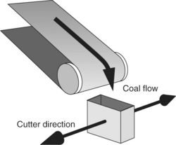

A cutter is passed at constant speed through the entire filling stream to collect the increment or divert an increment to a sample receival system. The width of the cutter is specified by ISO and Australian standards to be at least three times the nominal particle top size, while 2.5 times is specified in ASTM standards. Cutters that collect the increment before transferring it into a sample receival system must have sufficient capacity to hold all the increment without the chance of overflow. For falling steam samplers, the mass of increment collected is given by:
C is the coal flow rate in tonnes per hour,
b is the cutter aperture width, in millimetres,
vc is the cutter speed in metres per second.
Cross-belt cutters collect increments from the coal stream while it is being transported on a conveyor belt. The swinging cutter traverses the entire belt width taking all coal in its path. The set-up of the cross-belt samplers requires that the profile of the conveyor belt is closely controlled so that no coal is left on the belt as the cut is taken and the belt is not damaged in the process.
The mass of an increment taken by cross-belt sampler is given by:
C is the coal flow rate in tonnes per hour,
b is the cutter aperture width, in millimetres,
vb is the belt speed in metres per second..
There are practical limits to the cutter speed when using mechanical samplers. As such, the mass of increment collected can be much greater than the minimum mass required. This is especially the case where the coal flow rates are relatively high, as may be experienced with coal preparation plant product conveyors and ship loading conveyor systems.
The minimum increment mass is related to the number of increments required to constitute a sample, and is based on the required sampling precision and the sampling characteristics of the coal, namely IH and DH. ISO 13902–4 and AS 4264.1 nominate the minimum mass of sample for a given nominal top size of the coal to be sampled (Table 5.4) and also provide guidelines for calculating the number of increments and sublots.
Table 5.4
Suggested general analysis sample mass for different coal top size
| Nominal top size (mm) | General Analysis Mass (for approximate precision of 0.2% ash) (kg) |
| 300 | 15 000 |
| 200 | 5400 |
| 150 | 2600 |
| 125 | 1700 |
| 90 | 750 |
| 63 | 300 |
| 50 | 170 |
| 45.0 | 125 |
| 31.5 | 55 |
| 22.4 | 32 |
| 16 | 20 |
| 11.2 | 13 |
| 10 | 10 |
| 8 | 6 |
| 5.6 | 3 |
| 4.0 | 1.5 |
The minimum average increment mass to be collected in order to achieve the specified sampling precision is:
ms = the minimum total sample mass,
n = the minimum number of increments to be taken to form the sample.
A single-stage mechanical sampler collects the required number of increments from the falling stream or from the conveyor belt to form the sample and stores it in a container until it is collected and transported to the laboratory for processing.
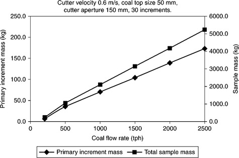
In the event the total sample mass collected by combining all the increments is so large that it is impractical to collect or to be handled by the laboratory, division or subsampling of primary increments can be incorporated in the sampling system as an additional stage. Figure 5.10 shows the relationship between coal flow rate, primary increment mass and total sample mass collected, when sampling 50 mm top size coal using a sampling system with a 150 mm aperture cutter moving at 0.6 m− 2. Clearly, under these circumstances, the mass of coal would become too large for practical purposes of handling, transport to the laboratory and laboratory processing once the coal flow rate exceeded about 200 tph.
Increment division must be conducted so that the integrity of the resultant sample is preserved and the precision requirements are met. Division is also a sampling operation, and the principles of sampling as covered earlier in this chapter apply. The sampling standards provide guidance on when and how increments should be taken. ISO5 specifies a minimum of four cuts or divisions per primary increment. ASTM8 and Australian Standards11 specify a minimum of six for the division of primary increments.
It is a requirement of ISO and Australian standards that the mass of the final sample after increment division must be no less than the minimum sample mass as specified by the standard for the top size of the coal and the type of analysis to be conducted (Table 5.4). In the case of coal with a 50 mm top size, the minimum mass for general analysis is 170 kg. On this basis, if 45 primary increments are required and each divided six times as per requirements of ASTM and Australian standards, the minimum mass of the combined divisions from each increment needs to yield 3.8 kg of coal or 0.63 kg per division.
In general, therefore, the mass of coal retained from dividing each primary increment must be no less than the minimum increment mass, which is defined as the minimum sample mass divided by the number of increments.
If the division of all primary increments by the minimum number of cuts per increment yields a total sample mass of more than the minimum sample mass required, then sample division is an option for reducing the sample mass without significant effects on precision. However, if the resultant sample mass is less than the minimum required mass, the primary increments must be crushed to reduce the top size before division. If the 50 mm coal used in the above example is crushed to a top size of 10 mm then, from Table 5.3, the mass of the sample required after combining the subsamples from each divided increment is 10 kg.
Primary increment flow rates at large coal handling facilities can be quite large. Kooragang Coal Terminal in Australia can load ships at the rate of 10 500 tph. As a ship is being loaded with coal, primary increments are extracted at a maximum rate of approximately one per 93 tonnes. The primary increment mass is approximately 300 kg and therefore the sampling facility has to have the capacity to handle a primary increment flow rate of approximately 34 tph. Division of primary increments is a necessity. Given the relatively high capital cost of a 34 tph crushing and handling plant, it is more cost effective to divide the primary increments before crushing.
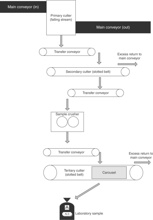
Figure 5.11 is a schematic of a tertiary sampling system similar to what may be found at modern coal loading facilities. A falling-stream sample cutter takes a primary increment at the transfer point on the main conveyor. The primary increment is transferred to a secondary cutter, in this case a slotted belt. Six cuts are taken for each primary increment. The secondary increments are transferred to a sample crusher. After crushing, the coal is transferred to a tertiary cutter which takes 12 divisions and deposits them into a canister in a carousel. When sampling is complete the canister is emptied and transported to the laboratory.
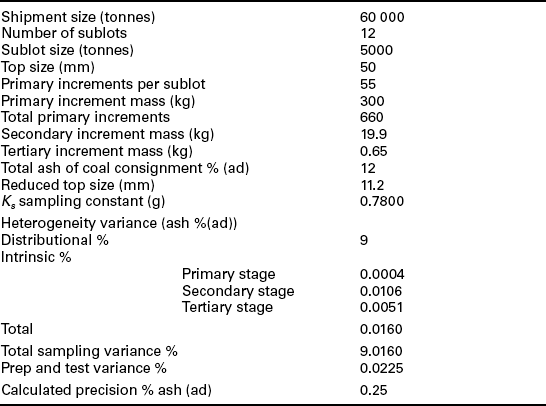
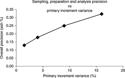
Analysis of the sampling process for a coal of known characteristics yields the overall precision of sampling, sample preparation and analysis. For the system in Fig. 5.10, sampling a shipment of 60 000 tonnes of washed product coal and assuming a variance of 9% (standard deviation 3% ash) the results of the analysis for each stage are presented in Table 5.5. Under these circumstances the overall precision for ash determination of the shipment is 0.16%. (Calculations were made using Equations [5.4]–[5.8].)
Large multi-stage sampling systems frequently have to deal with multiple coal types, especially those at multiuser shipping terminals. Therefore, they can be expected to have to handle coal types and coal flows of varying sampling characteristics, while at the same time producing an acceptable level of overall sampling variance. As a consequence, the sampling systems will then need to be designed for a reasonable worst case sampling scenario. Figure 5.12 shows the relationship of primary increment variance and overall precision for the sampling system given in Fig. 5.10 over a range of primary increment variance values from a relatively low value of 1.0% to a very high value 16.0% (representing standard deviations of 1% and 4% ash respectively). The precision is inclusive of contributions from sampling, sample preparation and analysis. The range of resultant precision values is 0.13–0.32% ash. It is expected that the greater majority of coal types would have sampling characteristics being sampled by this system would yield an acceptable precision value between about 0.15 % and 0.25%.
The analysis in Table 5.5 also clearly demonstrates that variance from DH can be expected to be dominant in systems characterised by large primary increment masses. The IH variance of primary, secondary and tertiary stages is almost insignificant compared to the variance from primary increment DH.
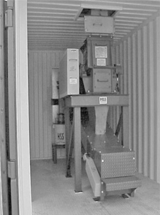
Figure 5.13 shows a single-stage cross-belt sampling system in place on a conveyor belt. Each primary increment taken by the cross-belt cutter is deposited directly into the sample container without further subdivision or crushing. These types of systems are relatively low cost but are suitable only for very low material flow rates and small particle top sizes.

5.13 A single-stage cross-belt sampling system with sample container carousel. (Courtesy of McLanahan Sampling Systems.)
Figures 5.14–5.16 are photographs of a two-stage sampling system. A cross-belt cutter (Fig. 5.15) extracts the primary increment from the main belt. The primary increment is transferred to the secondary stage housed in a small building (Fig. 5.16) where secondary increments are extracted and combined in a sampling container for laboratory collection. Excess primary increment, after the secondary increments have been extracted, is returned to the main conveyor via a transfer conveyor system.

5.14 Two-stage sampling system consisting of a cross-belt sampler, transfer conveyors, container housing the second-stage system and a transfer conveyor for returning excess sample to the main belt. (Courtesy of McLanahan Sampling Systems.)

5.15 Primary cross-belt sample cutter housing on a conveyor. (Courtesy of McLanahan Sampling Systems.)
5.16 Secondary stage of sampling system consisting of crusher, secondary cutter and sample container. (Courtesy of McLanahan Sampling Systems.)
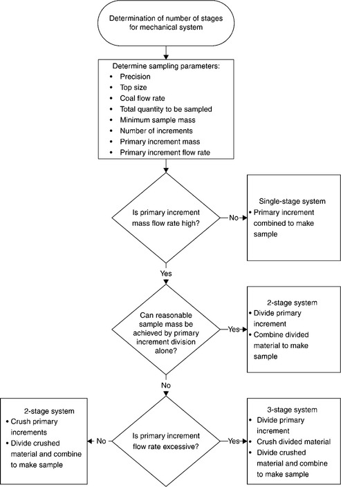
Selection of single, double or three stage mechanical system
The decision to select a single, two or three stage sampling system should be based on the sampling characteristics of the material being sampled, the material flow rates from which the primary increments are to be extracted and the level of precision required for the testing and analysis results.
Figure 5.17 gives an example of a decision process flow chart used for evaluating options.
5.4.2 Manual sampling
There are many instances where coal samples need to be collected but where there is no mechanical sampler available, for example when sampling process streams in a coal preparation plant. In such instances sampling needs to be done manually. This will usually involve the manual operation of a sampling implement such as a sampling ladle (Fig. 5.18). Ideally, increments will be collected from falling streams. Sampling standards specify how manual samples are to be taken. Some of the key points are:

• Safety is the prime consideration and a risk assessment needs to be conducted to identify risks to the sampling technician during collection of increments and while working in the area. Installation of guard rails and other measures may be required to make the area safe for sampling.
• The equiprobable sampling principle needs to be applied. The ladle (cutter) must traverse the whole coal stream at a constant (cutting) velocity. Coal stream discharging from conveyor belts, screens, vibrating feeders and chutes characteristically exhibit high levels of segregation and grouping. Failure to uniformly traverse the whole of the falling stream during collection of the increment has a high probability of introducing significant bias.
• The same cutting velocity must be used for all increments that are combined to make up a sample.
• The width of the cutter must be at least three times the nominal top size of the coal being sampled.
• The ladle is not to be overfilled. Where the coal flow rate is so large, or the width of the stream is so wide that it is physically impossible to collect an increment in a single pass, multiple passes may be made at successive positions across the stream to build up a single increment. The same number of passes will need to be made when collecting each increment.
• The minimum mass of the increment is to comply with the relevant standard.
Where a sample is required from a conveyor belt and there is either no access to a falling stream or the flow rate is too large for increments to be extracted manually, it may be possible to stop the loaded conveyor belt and to extract the increment directly from the belt. This is called stop-belt sampling. Stop- belt sampling is used for precision and bias testing of mechanical samplers as increments are able to be well delimited and the quantity extracted is relatively uniform for all increments. In this operation, the belt is stopped and a sampling frame is inserted through the coal bed so that it is in contact with the underlying belt. Coal particles that are obstructing the insertion of the frame are systematically moved, such that particles that are to the left of the frame are put into the increment while those to the right of the frame are not considered part of the increment. All coal particles within the sampling frame are included in the increment. The sampling frame should have an internal diameter at least three times the nominal top size of the coal. Stop- belt sampling is usually very disruptive to operations, especially considering that, ideally, thirty or more increments may be required to produce a sample for which the analysis will have acceptable levels of precision.
Sampling from stationary situations, such as stockpiles, wagons, trucks or ships’ holds, does not produce reliable samples. This practice should be avoided. Stockpiles can be effectively sampled only when the stockpile is being built up or broken down. Trains and trucks can only effectively be sampled from the falling stream after the material has been discharged and ensuring that the principle of equiprobable sampling is observed.
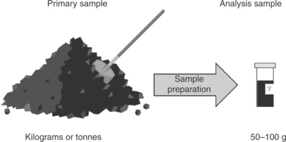
5.5 Sample preparation
The objective of sample preparation is to prepare test samples from a parent sample or individual primary increments, Fig. 5.19 for analysis. Sample preparation includes all procedures that a sample is subjected to in order to produce a reduced mass of sample (analysis sample) that is representative of the parent sample and from which subsamples of relatively small mass can be used directly for analysis. Samples for general analysis (proximate, ultimate, calorific value, total sulphur, etc.) are typically milled samples with 95% passing 0.212 mm. Standard AS4264.1 stipulates that the minimum mass required for general analysis is 30 g.
However, some laboratory analyses will require larger sample masses. Some examples from AS 4264.1 include Hardgrove grindability index (AS 1038.20) which requires 1 kg at 4.75 mm top size, and total moisture (AS 1038.1 – Method A and B) 300 g at 4 mm. However, the principles of preparing a representative analysis sample from the original coal sample are the same.
Taking the ash determination as an example: 1 g of coal is used in a single ash determination, and that 1 g has to be representative of the coal sample. At a top size of 0.212 mm the sampling constant, Ks, for most coals will be very small and this constant combined with a 1 g mass of coal enables the variance contribution from the IH of the analysis sample to be almost insignificant and therefore a high level of precision can be expected.
The goal of sample preparation has to be to produce the sample for analysis while maintaining acceptable levels of error, or simply, so that the result meets the required precision criteria.
Apart from exploration samples, most samples received by laboratories are from mechanical sampling systems at coal handling facilities at mine sites, ports or power stations. In some areas where coal is being sold across land boarders such as the Mongolian–Chinese border, most samples will be extracted directly from haulage trucks. Many samples, such as ship loading samples and some coal preparation plant samples, are produced by multistage mechanical sampling systems. Other samples may be produced from single-stage samplers. As a result, laboratories can receive samples in a wide range of conditions, most importantly sample mass, moisture content and particle size distributions. Sample preparation procedures have to be tailored to suit the samples and the proposed testing and analyses procedures that the sample has been collected for.
Sample preparation is usually divided into a number of stages with each stage consisting of
In some instances the particle size reduction may be omitted before sample subdivision, for example at the first stage after collection of the primary increment. However, generally before subdivision (subsampling) the particle size should be reduced.
Figure 5.20 shows the stages conducted by the laboratory on a gross sample.

In each case at every stage, the process recognises the relationships between the number of increments, sample mass and particle size to sampling variance, as each stage is a standalone sampling exercise.
Sample crushing
Jaw crushers, hammer crushers, roll crushers, hammer mills, disc mills and ring mills are typically used in laboratories for size reduction during sample preparation.
Jaw crushers
Jaw crushers comprise a fixed plate and a movable plate (Fig. 5.21). The gap between the plates can be adjusted to achieve the required top size.

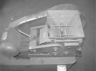
5.5.1 Hammer mills
Hammers mills comprise a set of swinging hammers attached to a rotating shaft (Fig. 5.22). Typically, they are fed a 4 mm top size coal to produce analysis samples with > 95% passing 0.212 mm. They have a device for feeding the coal into the mill. This is often a screw-type feeder. They also usually have a screen on the outlet to ensure that the entire sample achieves a specific top size. Hammer mills tend to generate excessive fines and should not be used in some instances, such as preparation of samples for petrographic analysis and Hardgrove grindability index determination.

5.5.2 Ring mills
Ring mills comprise a cylindrical canister and lid, a steel ring, and a smaller steel cylinder that fits inside the canister (Fig. 5.23). The coal is placed in the canister with the ring and the cylinder, and the lid is attached. This is then placed in a jig that moves the canister in a circular motion. The movement of the various metal components within the canister crushes the coal. There is some concern that these mills can become heated and that this may affect the coal quality, particularly CSN values. This type of mill is particularly useful for crushing low mass samples as sample loss is kept to a minimum. Automated ring mills have been in use in laboratories handling large sample volumes to ensure consistent milling and improved productivity.
5.5.3 Roll crushers
Roll crushers are comprised of two steel cylinders (Fig. 5.24). The coal is crushed as it passes between the cylinders. This type of crusher is useful when preparing samples with a minimum of fines generation.
5.5.4 Sample division
Sample division can be carried out using a number of methods including incremental division, rotary sample division, riffling, fractional shovelling and strip mix and splitting.
Incremental division
Incremental division is a manual method of subdivision that can provide precise subsamples. This method requires that the coal is well mixed prior to division. The coal is spread onto a flat surface in the form of a rectangle in a thickness approximately three times the nominal top size of the sample. A grid pattern is marked out on the sample (usually composed of at least 20 rectangles in a 5 × 4 grid) and a single increment is obtained from each square. The increment is removed from the sample using a suitable scoop and bump plate to prevent the increment from falling out of the scoop. Incremental division is used almost exclusively in obtaining the final (− 0.212 mm) laboratory sample after the hammer mill operation, because of excessive dust losses by other methods.
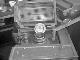
5.5.5 Rotary sample dividers
Rotary sample division (rsd) is the most common method for subdivision of large samples in coal laboratories. The rotary sample divider (Fig. 5.25) comprises a feed hopper, a device for feeding the coal at a constant rate (usually a vibratory feeder) and a number of sector-shaped canisters formed into a cylinder on a rotating platform. The uniform coal stream produces a falling stream of coal that is collected in the rotating canisters, dividing the sample into representative parts.
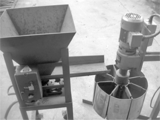
As the coal particles move through the feed hopper there is a high potential that some segregation and grouping will occur. To counter the effect that this may having on sample preparation variance it is advisable to ensure that each canister cuts the falling stream at least 20 times, i.e. there are at least twenty rotations of the turntable as the coal flows into the canisters. Additionally, it is a good practice to combine material collected in two or more canisters to form the divided increment or subsample. When doing so, canisters that are opposite each other in the rotary sample divider should be selected for recombination. The machine pictured in Fig. 5.25 is set to divide a sample into eight divisions. If the requirement was to extract a quarter of the sample for analysis, two of the 1/8th divisions would be recombined.
5.5.6 Riffles
Riffles (Fig. 5.26) are less regularly used in laboratories. Riffles divide the coal into halves by allowing the coal to fall through a set of parallel slots of uniform width. Adjacent slots feed opposite containers. The width of the slots should be at least three times the nominal top size of the coal. There should be at least eight slots for each half of the riffle.

5.5.7 Fractional shovelling
Fractional shovelling may be used for subsampling when a large rotary sample divider is not available. In this process, the coal is formed into a conical heap. Successive shovels of coal are removed from the base of the heap and are placed into daughter heaps. The shovels of coal should be allocated consecutively and systematically to each daughter heap.
5.6 Future trends
The evolution of sampling systems continues in parallel with computing technology and manufacturing technology. It is envisaged that with improved sampling technology sampling plant will become more affordable, reliable and smarter. This will probably include systems that monitor their own performance, such as velocity of cutters through coal streams. It is also possible that novel sampling plants will be developed for more process streams within coal preparation plants. Such streams could include discharge from product and rejects screens as well as various slurry flows.
Online analysers may compete with mechanical sampling plant to the point where sampling systems in some situations may become redundant. This would include coal preparation plant product streams, train loading systems and product receival systems, such as at power stations. Online analysers will still need to obey sampling principles, in particular the equiprobability of all particles being selected for analysis by the instrument. Online analysers have been in use for many years, but their acceptance has been mixed for various reasons. It may be only a matter of time before they are taken for granted at mine sites and large-scale coal handling plants, permanently displacing physical sampling plants and their inevitable laboratory service.
5.6.1 Sample preparation in the laboratory
Laboratory sample preparation lends itself to mechanisation and automation. Systems have been available for some time that can take much of the manual handling component out of sample preparation. These systems, for example, lift a container of coal and transfer the contents to a hopper. The coal is then fed to a crusher and sample divider that produces a sample ready for final milling. The remainder of the sample is bagged ready for reserving. It is not much of a step to automate this process so that many samples can be processed in a production line. However, these systems are relatively expensive and need a consistently high volume of samples to support the business case or the capital expenditure. Therefore they are most likely to appear in the larger laboratories.
Alternatively, the automated systems remove the need for skilled labour to conduct sample preparation and may be justified for remote laboratories where suitable labour is scarce.
Final milling of samples to produce sample ready for laboratory analysis is a routine task and even small laboratories can produce more than a hundred samples each day. Larger bore core laboratories can be expected to produce many more milled samples each day. Milling involves placing sample that has been crushed to say 4 mm top size into a swinging hammer mill (Fig. 5.22) or a ring mill (Fig. 5.23). After each sample the mill has to be cleaned ready for the next sample, so that contamination does not occur. Milling systems that are self-loading and self-cleaning are able to process samples faster and at lower cost than manually operated systems. To date there are very few of these systems in production. However, with the appearance of very large, high capacity laboratories, such as the bore core laboratory operated by ALS Ltd in Brisbane, Australia, and the drive to improve efficiencies, reduce sample turnaround times and ensure quality of results, more automated sample preparation systems will appear.
5.7 Conclusion
The purpose of this overview of the statistical description of the heterogeneity of coal has been to demonstrate the science behind sampling to emphasise that any sampling scheme for a coal needs to take into account the characteristics of the coal being sampled and the level of precision expected from the scheme. There are several key and practical conclusions that emerge for design, implementation and management sampling systems and programmes.
1. A number of increments are required to be taken from a consignment of coal, and are combined to form a sample. The increments should be taken at regular intervals, either time based or mass based, and combined to form the sample. The number of increments to be taken must be predetermined based on the desired level of precision and coal sampling characteristics either as calculated or as provided in one of the standards (ASTM, ISO, AS).
2. The larger the number of increments collected, the better the precision of the sampling.
3. The mass of each primary increment needs to be large enough to ensure that variance resulting from inherent heterogeneity is not a major component of the total sampling, preparation and testing error.
4. Variance from IH is proportional to the inverse of increment mass. To halve the variance, the mass collected must be doubled.
5. Variance from IH is proportional to the particle top size cubed. If the top size is doubled then the mass of sample to be collected needs to be changed by 23 or 8 times the original mass, assuming there are no liberation effects by reducing the top size by half. Generally the change in particle size is raised to the power of 2.8 instead of 3 to allow for liberation effects.
6. Variance due to IH with respect to ash % can be estimated from wash- ability data, as long as the washability data is from a sample that is reasonably assumed to be representative of the coal of interest.
7. Variance from distributional or long-term heterogeneity can be assessed only by measurement of the variation of the analyte of interest such as ash %, with time or mass handled. Measurement can be by online analysers or by taking and analysing separately, multiple increments from a moving stream of coal.
8. When designing a sampling system the designer is faced with making assumptions on variance due to both intrinsic and DH unless there is existing data for the coal and the coal system being sampled. Some Standards provide guidelines for sampling coal when the sampling characteristics of that coal are unknown.
9. The various statistical relationships examined can be applied to the analysis of existing sampling systems in order to assess the overall precision of analytical data derived from samples produced by the system.
10. Increments must be ‘cuts’ which traverse or intersect the whole width and depth of the coal stream, usually at a transfer point or through a falling stream of coal. This is done to ensure that every particle has an equal opportunity to be sampled (Fig. 5.27).
11. The sampling implement must intersect the stream of material at a constant velocity (Fig. 5.28).
12. The width of the sampling implement or cutter must be at least three times wider than the nominal top size (as opposed to top size) of the coal being sampled.
13. The increment must never overfill the sample collection container (Fig. 5.29).
14. The weight of the increment must be known. This is to ensure that a minimum number of particles are collected for each increment. However, the minimum mass of an increment should never be less than 100 g, except where it can be shown that there is no loss of integrity of the individual increment. The minimum increment should never be less than 35 g.
15. If the number of primary increments becomes too large to achieve the desired level of precision, sublots of the coal can be sampled and analysed separately and the results averaged in order to improve the level of precision.
5.8 References
1. Gy Pierre, M., Sampling of Particulate Materials; Theory and Practice. Developments of Geomathematics 4. Elsevier Scientific Publishing Company, Amsterdam, 1979.
2. Lyman, G.J., Principles of samplingSwanson, A.R., Partridge, A.C., eds. Advanced Coal Preparation Monograph Series, Volume II, part 4. Australian Coal Preparation Society, 1994.
3. Lyman, G.J., Principles of sampling and statistics. D., Edward, C., Clarkson. Final Report ACARP C3090. Assess Status and Potential Improvements to Accuracy of On-Line Gauges, 1999.
4. Pitard, F.F. Pierre Gy’s Sampling Theory and Sampling Practice, 2nd Edition. Florida: CRC Press; 1993.
5. International Standard ISO 13909 Parts 1 to 8, ‘Hard coal and coke – Mechanical Sampling of Coal’, International Organization for Standardization.
6. ASTM D7430–12. Standard Practice for Mechanical Sampling of Coal. West Conshohocken, PA: ASTM International; 2012.
7. Australian Standard AS 4264.1,2,3 and 5 ‘Coal and Coke Sampling’, Standards Australia.
8. ASTM D2244/D2234M-10 ‘Standard Practice for Collection of a Gross Sample of Coal’, ASTM International, West Conshohocken, P.A.