
Optimization, simulation and control of coal preparation plants
Abstract:
Coal preparation plants incorporate a variety of separation processes that operate in relatively independent parallel circuits. The identification of optimum cutpoints for each circuit that globally maximize plant performance have historically involved the use of mathematical simulation routines. Unfortunately, these routines require detailed washability data and empirical partition information that is not always available to plant operators. In addition, fluctuations in the washability characteristics of the plant feed often make this approach impractical to implement in modern plants. This chapter suggests a more practical approach to plant control that involves generic operating protocols based on fundamental scientific principles that operators can adopt to optimize plant performance. Several industrial case studies are also presented that demonstrate the economic impacts of these optimization strategies.
17.1 Introduction
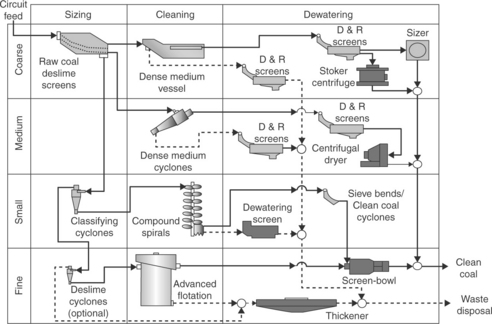
The flowsheet for a coal preparation plant can typically be represented by a series of sequential unit operations for sizing, cleaning, and dewatering (Fig. 17.1). This sequence of steps is repeated for each size fraction, since the processes used in modern plants have a limited range of applicability in terms of particle size (Osborne, 1988). As a result, modern plants may include as many as four separate processing circuits for treating the coarse (+ 50 mm), small (50 × 1 mm), fine (1 × 0.15 mm), and ultrafine (− 0.15 mm) material (Kempnich, 2000). Plant operators must select appropriate cutpoints for each cleaning process to ensure that the overall clean coal product from the plant meets quality criteria dictated by sales contracts. Plant operators often incorrectly select cutpoints that produce the same clean coal quality in every circuit throughout the plant. While this approach guarantees that the target quality is met, this method usually does not provide the highest overall yield of clean coal.
Historically, mathematical simulation routines have been used to identify optimum cutpoints (Armstrong and Whitmore, 1982; Peng and Luckie, 1991; King, 1999). The simulations are conducted using experimental float–sink data for different size fractions of the feed coal and partition curves for the different separation processes. The simulations are repeated for all possible cutpoints for each circuit and the combination that provides the highest plant yield at the desired target quality is selected as the optimum. Unfortunately, simulation routines require detailed washability data and empirical partition information that is not readily available to most plant operators. This approach is also impractical to implement in modern coal cleaning plants, since the feed coals are usually subject to significant variations in size, quality, and mineralogical association.
This chapter discusses some of the fundamental underlying principles that influence the optimization of coal preparation facilities. In the light of these principles, practical operating guidelines are provided that can be adopted by plant operators to effectively maximize clean coal yield. These guidelines, when combined with properly applied data from mathematical simulation routines, provide operators with critical information necessary to ensure that the plant product meets customers’ requirements while simultaneously providing the highest level of profitability. Several site-specific examples are presented to demonstrate the large potential financial impact of these important optimization guidelines.
17.2 Yield maximization
The objective of coal preparation is to separate valuable coal from unwanted mineral matter. Separation is achieved by exploiting differences in the physical (e.g., density, size, shape) and physico-chemical (e.g., wettability) properties of coal and mineral matter. Ideally, the plant-wide separation should be as efficient as possible in order to maximize coal yield at a given quality specification. In fact, it is often possible to improve the efficiency of a given plant by selecting the proper separating points for treating one or more feed coals.
17.2.1 Blending calculations
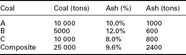
The first step in the yield maximization procedure requires that the quality (i.e., ash, sulfur, etc.) of combined streams from various plant circuits be mathematically calculated. This process, which is commonly called coal blending, involves simple weighted averages. For blending of multiple coals, blending calculations are best performed using the simple tabular format shown in Table 17.1. The total ash content of the mix is calculated by dividing the total tons of ash by the total tons of coal (i.e., 2400/25 000 = 0.096 = 9.6%). Simple weighted averages can be used to calculate a variety of common assays for mixed coals such as ash, sulfur, calorific value (kcal/kg), moisture, and so forth. However, mixing for the purpose of obtaining coal blends of desired chemical properties (e.g., ash fusion temperature, free swelling index, etc.) requires extensive knowledge and expertise and cannot be undertaken using this simple approach because these coal quality parameters are not additive.
17.2.2 Direct approach for maximizing yield
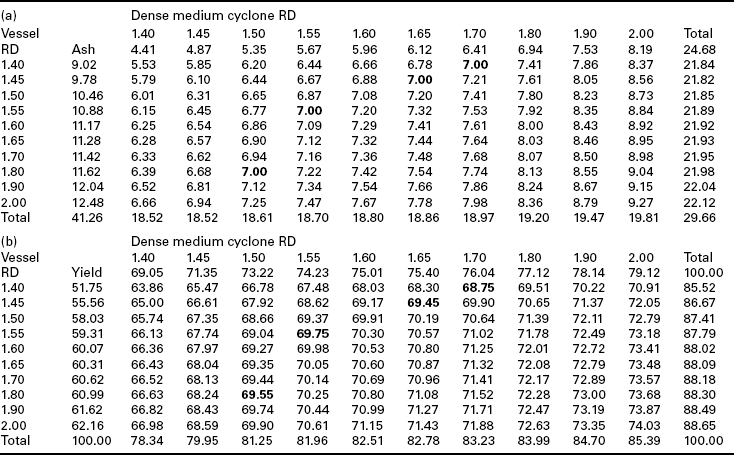
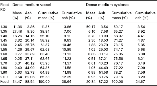
Blending calculations for coal preparation facilities can become complicated since the operating cutpoints in each circuit can be varied to generate clean coal products of different qualities (Mahr, 1981). Ideally, the cutpoints should be set to maximize the overall clean coal yield while still meeting the contract specifications. This concept is known as optimization. The oldest and most common optimization technique involves the calculation of all possible combinations of clean coal yield as a function of clean coal quality (Peng and Luckie, 1991). This approach can be demonstrated using a simple plant equipped with dense medium vessel and dense medium cyclone circuits. Simulated yield-ash values for the combined circuitry are summarized in Table 17.2 for all possible combinations of density cutpoints from 1.4 to 2.0 RD. For a target ash content of 7%, the highest attainable yield of 69.8% was obtained when both circuits were operated at 1.55 RD. No other combination of RD values provides a higher combined plant yield at this particular ash level. Interestingly, the optimum operating point corresponds to RD values that produce very different ash values in the individual dense medium vessel (10.9% ash) and dense medium cyclone (5.7% ash) circuits. Most industrial coal facilities are operated to produce the same cumulative product quality in all circuits, which is rarely optimal.
17.2.3 Maximizing yield via constant incremental quality
While the direct approach to plant optimization is theoretically correct, this trial-and-error methodology provides little insight regarding why a particular set of operating conditions is optimal. A better approach is to optimize circuits using the concept of constant incremental quality. This longstanding principle (Mayer, 1950; Dell; 1956; Abbott, 1982; Rayner, 1987) states that the maximum clean coal yield for a plant is obtained when all circuits are operated at the same incremental quality. In layman’s terms, incremental quality can be thought of as the effective quality of the last lump of material recovered (or discarded) in a circuit when the yield is increased (or decreased) by an infinitesimally small amount. Incremental ash content is typically the appropriate measure of quality for metallurgical coal plants, while incremental heat or energy value (BTU/lb or kcal/kg) is a more appropriate measure of quality for the thermal coal or steam coal market (Bethell et al., 2006).
Mathematical proof of the incremental quality concept is relatively straightforward and has been presented elsewhere (Luttrell et al., 2003). However, the fundamental basis for this concept can be demonstrated using the simple illustrations provided in Fig. 17.2. In both the upper and lower diagrams, the same two feed streams (A and B) are to be treated. The two streams could represent feed coal to two different cleaning operations in the same plant, the feed streams to two different plants that both service the same customer, or the same cleaning unit at two different points in time. The feed coals comprise various amounts of carbonaceous matter (black) and ash-bearing matter (gray). The washability of Stream A makes it relatively easy to upgrade since most of the particles are well liberated. In contrast, Stream B has a difficult washability due to the presence of a large percentage of middlings (composite particles).
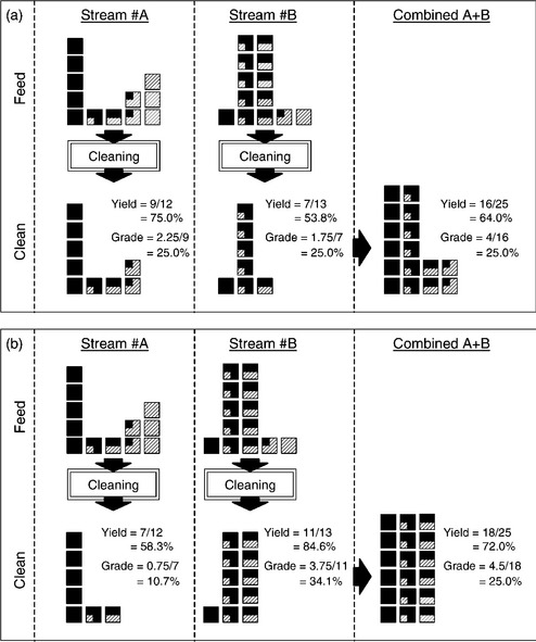
Figure 17.2 Clean coal products obtained by (a) treating parallel streams at constant cumulative ash, and (b) treating parallel streams at constant incremental ash.
The upper portion of Fig. 17.2 shows the result obtained when the separation is conducted to provide an identical target ash content of 25% for both streams. For Stream A, the operating point is raised from left to right until a total of nine units (blocks) are recovered out of a total of 12 units. This operating point produces a yield of 75% (i.e., 9/12 = 75%) at the desired target ash of 25% (i.e., 2.25/9 = 25%). For Stream B, a yield of only 53.8% (i.e., 7/13 = 53.8%) can be realized before the target ash of 25% (i.e., 1.75/7 = 25%) is exceeded. The lower yield is due to the poorer liberation of feed Stream B. The clean products from these two streams are blended together to produce a combined yield of 64% at the desired target ash of 25%. At first inspection, this appears to be an acceptable result since the target grade is met. However, a closer examination shows that particles containing 75% ash reported to clean coal when treating Stream A, while at the same time many particles containing just 50% ash were discarded when treating Stream B. This combination is obviously not optimum, since higher quality particles were discarded so that poorer quality particles could be taken.
The lower portion of Fig. 17.2 shows the result obtained when the separation is conducted such that the last unit of mass recovered in both cases contains 50% ash. This combination of operating points decreased the ash content of Stream A to 10.7% and increased the ash content of Stream B to 34.1%. However, when the two streams are blended together, the combined clean coal product still meets the required target ash of 25%. More importantly, this new set of operating points provides a higher combined yield (i.e., 72% vs 64%). In practice, it is easy for plant operators to be misled into accepting the lower yield because of the presence of multiple feed streams. The optimum result would be intuitive, however, if the feed streams had been blended together prior to cleaning. In this case, the pure black particles would be recovered first, then the 25% ash particles, then the 50% ash particles, and so on until no additional particles could be taken without exceeding the target ash. Obviously, this sequence will always provide the maximum recovery of valuable material at a given quality. As such, the incremental quality concept dictates that the maximum yield can be obtained only when the quality of the last unit recovered from each feed stream is identical.
17.2.4 Correlation with relative density
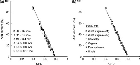
Incremental quality is a mathematical parameter that cannot be directly monitored in most industrial systems. However, this theoretical value can be estimated for ideal separations if the quality parameter of interest is ash. This approximation is based on the assumption that run-of-mine coals contain only two components: a low-density mineral-free carbonaceous component and a high-density pure-mineral component. Based on this assumption, the quality composition (Q) of a given particle must increase linearly with the reciprocal of particle density (ρ) according to the expression:
where RD1 and RD2 are the relative densities of the light (carbonaceous) and the dense (mineral) components, respectively, and K1 and K2 are fitting constants (Anon., 1966; Abbot and Miles, 1990).
The validity of the linear relationship expressed in Equation [17.1] can be demonstrated by plotting the ash contents of narrowly partitioned density fractions of coal obtained from standard float–sink tests. For example, these values are plotted in Fig. 17.3a for six different size fractions of a run-of- mine coal. For particles coarser than 0.6 mm, the data show that the same incremental ash is obtained for a given RD regardless of the size fraction treated. The slight deviation noted for the fractions finer than 0.6 mm can often be attributed to inefficiencies in the experimental float–sink procedures. Likewise, Fig. 17.3b shows that the linear relationship even holds for coal samples from different coal-producing regions (albeit slightly different linear relationships may be observed for bituminous coals of different rank due to density variations in the organic matter). The impacts of these variations must be evaluated on a case-by-case basis. The presence of a third density component (e.g., pyrite) in some coal fractions has also been known to create minor deviations from the linear relationship. Since Equation [17.1] shows that incremental ash is fixed by density, the incremental quality concept can now be extended to state that total plant yield is maximized by operating all circuits at the same relative density (Clarkson, 1992). This statement is true regardless of the size distribution or washability characteristics of the feed coal, provided that very efficient separations are maintained in each circuit (Luttrell et al., 2000). Obviously, separations that are driven by other constraints, such as sulfur limitations, need also to consider this quality parameter when targeting a specific incremental quality (Gupta and Mohanty, 2006).
17.3 Circuit simulation
Plant optimization would be relatively easy were it not for the presence of misplaced particles. A plant equipped with ideal separators could achieve optimum performance for ash removal simply by maintaining the same RD cutpoint in all parallel circuits. Unfortunately, this approach must be modified since ideal separators do not exist in practice. The impact of inefficiencies on the selection of optimum circuit cutpoints can be studied using a variety of mathematical techniques. The most common approach is to convert the ‘ideal’ separation curves obtained from standard characterization tests (e.g., float-sink tests) into ‘actual’ separation curves using empirical partition models (Armstrong and Whitmore, 1982; Rong and Lyman, 1985). The optimum RD cutpoints can then be identified using simulation programs equipped with an optimization engine (King, 1999). As described below, approximate rules of thumb can also be developed from these simulations to assist operators in quickly identifying optimum cutpoints for coals with different washability that may be passed through processing facilities (Luttrell et al., 2003).
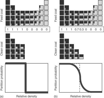
17.3.1 Partition modeling
Partition models are used to estimate the probability that a particle of a given RD will report to the clean coal stream. For example, when a coal is passed through a ‘perfect’ density separator (Fig. 17.4a), all particles with densities below the cutpoint (RD50) will be recovered to clean coal (P = 100%). Likewise, all particles with densities above the RD50 cutpoint will be rejected (P = 0%). In the real world, however, separations are never ideal and some particles get misplaced (Fig. 17.4b). This inefficiency causes the partition curve to flatten and deviate from ideal. (Note: In some countries, partition curves are plotted as RD vs the probability of reporting to refuse. This convention provides a mirror image of the partition curve based on clean coal partitioning.) The steepness of the partition curve, which reflects the sharpness of the separation, is typically reported using an Ecart Probable (Ep) value defined as:
in which RD25 and RD75 are the relative densities that correspond to probabilities of 25% and 75%. A lower Ep is desirable, since it means that fewer particles are misplaced during the separation.
Several detailed methods have been reported in the literature for establishing partition curves (Luckie et al., 1969). However, the fastest and simplest method involves the collection of representative samples of the feed, clean and refuse streams around the cleaning unit. Once collected, the samples are dried and representative splits subjected to ash analysis. From the ash values, the ratio (Z) of reject tonnage to clean tonnage can be calculated using:
in which f, c, and r are the feed, clean, and refuse ash contents, respectively. For example, the Z ratio for a dense medium separator coal treating a 25% feed ash and generating a 10% clean ash and 70% reject ash would be:
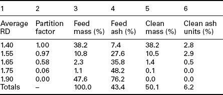
This calculation indicates that 0.333 tons of reject would be generated for each ton of clean coal. Representative splits of clean coal and refuse are then subjected to float–sink (washability) testing. The float–sink tests provide the mass percent of dry solids present in each density fraction. The first three columns of data in Table 17.3 (Columns 1–3) provide an example of the types of data obtained from such an exercise. From these data, the partition factor (P) for each density class can be quickly calculated using:
Table 17.3
Example of calculations for partition curve construction

in which R and C are the respective weight percentages of reject and clean coal in each density class. In this case, the partition factor (P) represents the probability that material of a given density in the feed will report to clean coal. These values, which are listed in Column 4 for the example shown, were calculated as follows:
As shown in Fig. 17.5, the partition curve for the separator can be constructed by plotting the partition factors (Column 4) as a function of the average RD of each class (Column 1). For the example shown, the cutpoint (RD50) is 1.66 RD, which corresponds to particles having an equal chance of reporting to either the clean or reject streams. The Ep value is 0.04 (i.e., (1.70 – 1.62)/2 = 0.04), which can be compared with tabular values, such as those shown in Fig. 17.6, to determine whether the level of performance is acceptable for the equipment and size fraction being evaluated.
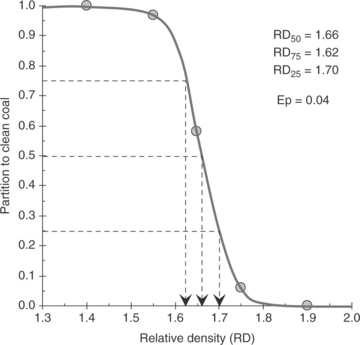
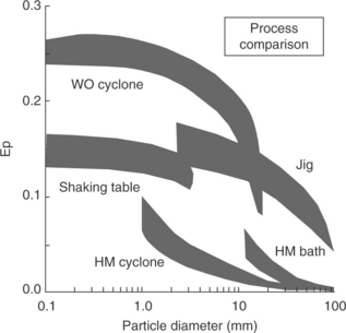
Figure 17.6 Approximate Ep values for coal cleaning equipment. (Source: After Osborne, 1988.)
17.3.2 Process simulation
Experimental partitioning data can also be used as the basis for predicting the effects of changes in feed coal washability on the performance of a separator. This is accomplished by simply multiplying the respective partition factors by the float–sink data for the new feed sample. The values for the individual classes can be cumulated to obtain the overall performance. For reference, an example of such a calculation is provided in Table 17.4 for the partitioning data plotted in Fig. 17.5. These calculations inherently assume that the partition curve is independent of the feed coal washability. This assumption is often not valid for water-based density separators in which particle–particle interactions influence the partitioning response (Tavares and King, 1995). For these unit operations, the overall shape of the partition curve can also be greatly impacted by water splits and other operational parameters (King, 2001; Rao, 2004).The approach can also introduce significant discretization errors if the upper and lower RD ranges for any density class are too large (Mohanta and Mishra, 2009). Therefore, considerable care should be exercised when applying partitioning data from one operation to another application.
Table 17.4
Example of calculations for partition curve simulations
Columns 3 and 4: Feed Coal Float – Sink Data.
Despite the potential pitfalls, partition modeling is still the most widely used method for plant design and performance prediction. Several software programs that can be used for this purpose are commercially available. These alternatives include well-known packages such as LIMN, METSIM, and MODSIM, as well as custom programs created by a wide variety of individuals and companies (Rong, 1992). In most cases, the simulation routines make use of empirical partition functions that belong to a mathematical family of transition functions (Scott and Napier-Munn, 1992; King, 2001; Rao et al., 2003). Examples of several such functions are listed in Table 17.5. Statistical regression methods are commonly used in a trial-and-error fashion to obtain the best possible fit between the experimental partition data and one of the empirical expressions. Depending on the particular application, one or more fitting equations may be appropriate. If such experimental data are not available, then the Ep values may be estimated using a procedure recommended by Osborne (1988), i.e.:
Table 17.5
Common transition functions used for partition curve fitting
| Function type | Mathematical expression |
| Exponential sum | P = [exp(αX) – 1]/[exp{αX} – exp{α} – 2] |
| Sigmoid (whiten) | P = 1/[1 + exp{α (1 – Z)}] |
| Weibull | P = 1 – exp{− ln(2)Zm} |
| Modified weibull | P = exp{− ln(2)/Zm} |
| Logistic response | P = 1 – 1/[1 + Zm] |
| Tangent | P = artan{α(X – 1)}/π – 1/2 |
in which f1, f2 and f3 represent factors that account for variations in Ep due to particle size, equipment size, and manufacturer’s guarantee (usually 1.1–1.2), respectively. Es is calculated using one of several standard functions. Table 17.6 lists some examples of these functions for different types of coal cleaning equipment.
Table 17.6
Examples of models used for partition simulations
| Separator type | Expression for Es | Typical f1 values |
| Baum jig | 0.78(RD50(RD50 – 1)) + 0.01 | 3 for 1 mm 0.5 for 100 mm |
| Dense medium vessel | 0.047RD50 – 0.05 | 0.5 for coarse 1.4 for small |
| Dense medium cyclone | 0.027 RD50 – 0.01 | 2 for 0.5 mm 0.75 for 10 mm |
| Water-only cyclone | 0.33RD50 – 0.31 | Depends of particle size and washability |
| Spiral separator | RD50 – 1 | Depends of particle size and washability |
Source: After Osborne, 1988.
Unfortunately, the partition simulation approach can be a complicated exercise that requires substantial expertise and knowledge. As such, this task should be assigned to technical staff who are properly equipped with the computing facilities and staff needed to successfully perform these calculations. Optimum RD50 values identified from simulation work may not be attainable in practice due to equipment limitations. For example, many water-based separators such as spirals can operate only at relatively high RD cutpoints. Therefore, these limitations must also be taken into account when plant design work and optimization studies are performed. Experienced plant design engineers and equipment vendors should be consulted whenever possible to clearly identify the cost and production constraints associated with equipment performance limitations.
17.3.3 Impacts of misplaced material
Due to the lack of detailed data and skilled personnel necessary for day-to- day plant simulations, plant operators are often forced to resort to approximate methods for plant optimization. For example, Fig. 17.7 shows the results of performance simulations conducted using a hypothetical set of float–sink data for coarse (50 × 1 mm) and fine (1 × 0.15 mm) cleaning circuits. The plots show the total plant yield as a function of the difference between the relative density cutpoint (RD50) of the coarse and fine circuits (i.e., difference in RD50 = fine RD50 – coarse RD50). In Fig. 17.7a, simulations were conducted using identical Ep values (either 0.02 or 0.07) for both the coarse and fine circuits. In Fig. 17.7b, the Ep for the coarse circuit was held constant at 0.02, while the Ep for the fine circuit was varied over three values (0.02, 0.07 and 0.14). Several important observations can be made from the simulation data. The first and most obvious is that separation efficiency has a large impact on total plant yield. Figure 17.7a and 17.7b both show a drop in yield of several percentage points as the Ep becomes worse. The second observation, which was discussed in the previous section, is that maximum plant yield is achieved when all ‘similarly efficient’ circuits cut at the same RD50. As shown in Fig. 17.7a, the maximum yield occurs when the RD50 in both the fine and coarse circuits are identical (i.e., difference in RD50 is zero). This result should be expected given the previous discussion related to optimization via operation at constant incremental quality. The third observation, which is often overlooked by plant designers and operators, is that inherently less efficient circuits, such as most common water-based separators, must be designed to cut at a slightly higher RD50 in order to maximize plant yield. For the case shown in Fig. 17.7b, the fine circuit operating at Ep = 0.14 must cut about 0.1 RD units higher than an efficient coarse circuit operating at Ep = 0.02 to ensure that maximum yield is attained. Misplaced material associated with a poorer Ep has the effect of lowering the incremental ash of a product generated at a particular separating density. This is because the mass present in typical run-of-mine coals increases with decreasing specific gravity in the region where most industrial separations occur (i.e., below ≈ 1.7 SG). Consequently, a greater proportion of lower density middlings is misplaced into the refuse stream than higher density middlings into the clean coal stream. The shift of higher quality (lower ash) material lowers the effective incremental ash. Therefore, less efficient circuits must be operated at a higher density cutpoint in order to maintain the same incremental quality (Clarkson, 1992; Luttrell et al., 2003). Since efficiencies of density-based separators tend to decline as the particle size decreases, circuits treating finer particles must typically use correspondingly higher RD50 values to maximize total plant yield.

Figure 17.7 Total plant yield as a function of difference in RD50 for (a) identical Ep values and (b) different Ep values in fine and coarse circuits.
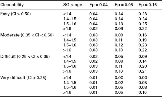
The degree to which the RD50 must be increased for less efficient processes can usually be determined in advance using simulation software and then tabulated in a simplified format for plant operators. To simplify the tabulation, coal types need to be classified according to their washing potential using a cleanability index (CI). The index, which can vary from 0 to 1, is mathematically defined as:
in which Y1.3 and Y1.6 are the clean coal yields obtained from the washability data at density values of 1.3 and 1.6 RD, respectively. Obviously, a feed coal that responds well to density separations would have a very high CI value, while a poorly responding feed coal would have a low CI value. In most cases, only four general categories of relative cleanability need to be established to distinguish coals with different washability characteristics: easy (CI > 0.50), moderate (0.35 < CI < 0.50), difficult (0.25 < CI < 0.35), and very difficult (CI < 0.25). For each generic type of coal feed to the plant, approximate corrections can then be established for different RD50 ranges and Ep values. Table 17.7 shows one such chart compiled for a small coal preparation facility. These corrections indicate in absolute points how much the RD must be increased in order to maintain the same incremental ash that would be obtained using an ideal separator at a given RD50. For example, this chart also shows that a 1.55 RD50 separation characterized by Ep = 0.08 and moderate cleanability (CI = 0.45) would need to operate at 0.23 SG points higher than an efficient separator to maintain the same incremental ash. This approximate method for plant optimization is useful since full numerical simulations to determine optimum cutpoints are impractical in most industrial situations due to constantly changing feed blends. However, this is only an estimation procedure, and significant errors may occur as a result of unexpected variations in feed coal washability or separator characteristics that may make these predictions less reliable.
17.4 Industrial case studies
The importance of the optimization strategies discussed in this chapter can be best illustrated via several industrial case studies. Examples have been provided for a diverse range of issues such as dense medium cutpoint selection, real-time quality control, equipment upgrade justifications and plant moisture reduction.
17.4.1 Dense medium circuit cutpoints
A case study was conducted for the dense medium circuits in one module of a large coal preparation facility. The circuitry included a single dense medium vessel that treats 300 TPH of plus 10 mm feed coal and a bank of dense medium cyclones that treats 700 TPH of 10 × 1 mm feed coal. The washability data for the feed coals supplied to each circuit are summarized in Table 17.8, but are not available to the plant operators. According to the production records at the plant, the operators routinely adjust the RD cutpoints to maintain the same clean coal ash of 7% from both the vessel and cyclone circuits. Because the coarser coal is less liberated, the vessel RD50 must be set to a low value of 1.3 RD in order to meet the 7% ash constraint, while the coal fed to the dense medium cyclone circuit is much better liberated and, as such, must operate at a much higher cutpoint of 1.75 RD to maintain the same 7% product ash.
Based on the optimization guidelines outlined above, the overall performance of the combined circuits cannot be optimum. For efficient units such as dense medium separators, total plant yield is maximized only when all parallel circuits are operated very near the same RD50. The large difference in RD50 between the vessel and cyclone circuits indicates that a better set of operating points is available. In fact, this problem can be observed by comparing the qualities of the last particles recovered in each of the two circuits. When operating at a cumulative ash of 7% (RD50 = 1.35), the last increment of mass recovered in the vessel circuit contained approximately 8.3% ash. To achieve the same cumulative product ash of 7%, the cyclone circuit had to be operated at a much higher cutpoint (RD50 = 1.75) and the last increment of recovered mass contained about 44.5% ash. The combined plant is obviously not optimum since one circuit is sending particles with more than 8.3% ash to reject, while the other is sending particles with less than 44.5% ash to the clean coal product.
The financial impact of the decision to operate at a constant cumulative ash as opposed to constant incremental ash can be estimated from the wash- ability data given in Table 17.8. For constant ash of 7% from both circuits, the combined clean coal tonnage will be:
Likewise, the results obtained by operating at constant incremental ash can be calculated for cases in which the RD cutpoint is held constant in both circuits. In this particular situation, operation of both circuits at a 1.55 SG provides the following clean coal ash and production rate:
These calculations show that the plant can increase overall tonnage by 50 TPH without impacting clean coal quality simply by maintaining the same RD50 in both circuits. This results in a net increase in saleable tonnage and profitability of about 7.6%. Also, operation at a constant RD is a much easier condition to maintain since the plant operators are constantly aware of the RD values, but rarely have access to the feed washability data.
17.4.2 Real-time quality control
Optimization via constant incremental quality also has significant implications on the protocols used for real-time control of coal preparation facilities; for example, the management of a large coal operation recently installed an on-line analyzer to monitor the ash content of their clean coal products. The analyzer was deemed necessary because of large fluctuations created by the intermittent addition of lower quality coal from a strip mining operation that frequently entered with the normal plant feed. The control loop was designed to automatically raise the RD cutpoints whenever the plant product ash was below 7.5% and drop the RD cutpoints whenever the ash was above 7.5%. Once the analyzer was properly calibrated, the plant management found the control system to provide a clean coal product with a very consistent quality. Therefore, the capital expenditure of more than $1 million for the on-line analyzer and associated ancillary controls was believed to be well justified.
Unfortunately, the control system described above is less than optimal, since it does not allow a constant incremental quality to be maintained. In fact, the control system is specifically designed to be less than optimal, since the programming logic constantly adjusts the RD cutpoints in response to variations in the feed coal washability. According to the incremental quality concept, plant performance can be optimized only by operating all efficient circuits at the same RD cutpoint. This requirement is valid not only for a fixed point in time, but also for the entire duration of a given production cycle. As such, a plant that raises and lowers RD cutpoints for quality control purposes will always produce less clean coal than a plant that maintains the same cutpoints. One viable approach to maintain constant cutpoints is to use the on-line analyzer to adjust the ratios of the feed coals entering the plant. In this approach, different feed coals are stored in separate stockpiles according to their general washability characteristics (Fig. 17.8). Based on feedback from the on-line analyzer, different ratios of coal from the piles can be automatically fed to the plant as required to maintain a constant clean coal quality for the overall product. The required feed rates can be controlled automatically using ratio feeders and a control loop, or they can be set manually via communication between the plant operator and the stockpile dozer worker who controls how much of each coal is directed to the plant. This approach allows the quality of the clean coal to be adjusted on-line without changing the predetermined cutpoints that optimize plant performance. Precise determination of the washability characteristics of the different coal feeds is not required since the control scheme determines the required mix ratios in real time. The feed coals simply need to be placed into separate piles with generally better and worse washability.
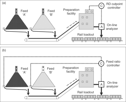
Figure 17.8 Quality control strategies based on (a) adjustment of RD cutpoints and (b) adjustment of feed coal blends.
The financial benefits of this approach can be illustrated by comparing production data obtained from the plant while operating under either RD control or feed ratio control. To fairly compare these two strategies, a series of plant simulations were performed over a production period of 24 h. The simulations were performed using ‘poor’ and ‘good’ plant feeds determined from statistical analyses of the plant feed coals. As expected, the simulation data showed a control system that employs a traditional on-line ash analyzer to maintain a constant product ash of 7.5% via on-line adjustment of RD cutpoints produced 7787 tons of saleable coal, while the simulation runs performed using the optimal ratio feeding control strategy produced 8133 tons of saleable coal at the same 7.5% ash. The use of the feed ratio control strategy increased the tonnage of saleable coal by 346 tons for this 24 h period. This improvement represents an increase of more than 14 TPH of marketable coal, which would typically pay for the required feed blending systems in less than a year.
17.4.3 Justification of equipment upgrades
The fundamental insight into plant optimization provided by the incremental quality concept can also be used to conduct first-pass evaluation of equipment upgrades within the coal preparation facility. For example, test data obtained from an industrial plant showed that the single-stage spirals were operating at RD50 = 1.95. To maintain a product quality, the dense medium cyclones were forced to operate at RD50 = 1.52. Information published in the literature showed that two-stage compound spirals can substantially reduce the resultant RD50 (Luttrell et al., 2007). Subsequent tests conducted in the plant showed that the addition of a second stage of cleaner spirals would reduce the cutpoint for the combined spiral circuit to RD50 = 1.75 and drop the clean coal tonnage from 62 TPH for the single-stage spirals down to 56 TPH for the two-stage spirals. As a result, the plant management decided to abandon the upgrade because such a move would result in 6 TPH less saleable coal from the spiral circuit. Unfortunately, this viewpoint fails to recognize that the global clean coal production is not optimized, due to the very large difference in the RD cutpoints between the dense medium cyclones and spirals. In the absence of more detailed information, the generic data given in Table 17.7 suggest that the spirals would need to operate at about 0.23 RD units higher than the dense medium cyclone to maintain an acceptable incremental ash. This value suggests that the two-stage circuitry would be preferable, since it provides a cutpoint near this value.
In this example, management failed to consider the impacts of reducing spiral RD50 on the overall plant production. A detailed examination of the test data showed that the drop in RD50 from 1.95 to 1.75 RD effectively reduced the incremental ash from about 62% to 38% in the spiral circuit. Although this action reduced the amount of saleable coal by about 6 TPH, the tonnage loss was largely due to the rejection of high-ash particles. The removal of high-ash material made it possible to raise the RD cutpoint in the dense medium circuit from 1.52 to 1.57 RD without exceeding the contract ash limit. The test data showed that the increased cutpoint raised the incremental ash in the dense medium circuits from about 25% to 34% which, in turn, increased the clean coal production from the dense medium circuit by 16 TPH. This provides a net gain in saleable tonnage for the overall plant of about 10 TPH when using the two-stage spirals. The higher net production from the two-stage spiral installation would typically provide a payback period of only a few months. Moreover, the plant moisture would typically be reduced somewhat, since a larger amount of coarser coal now makes up the combined product.
17.4.4 Benefits of improved dewatering
Moisture is an important consideration in all coal preparation facilities (Osborne and Davis, 1995). In fact, the incremental quality concept effectively governs how moisture and ash should be shifted between circuits to optimize the performance of coal blends sold to the stream market (Bethell and Luttrell, 2005; Bethell et al., 2006; Luttrell et al., 2009). This trade-off can be best illustrated by means of a simple case study conducted for an actual coal preparation facility. Table 17.9 compares three different scenarios for the operation of the facility that includes a dense medium vessel, dense medium cyclones and froth flotation. The clean coal is currently sold with a contract limit of 12 500 BTU/lb. In the baseline case (Case I), the plant circuits were all operated under optimum conditions using conventional dewatering equipment. The product moistures for the vessel, cyclone, and flotation circuits were held constant at 2.5%, 6.5%, and 25%, respectively. The maximum production that could be achieved while maintaining a 12 500 BTU/lb product was 728.4 TPH of clean coal (as-received basis). The optimum production occurred at a total incremental inert (ash plus moisture) content of 31.76% for all circuits. The clean coal moisture and ash contents were 7.48% and 9.29%, respectively.
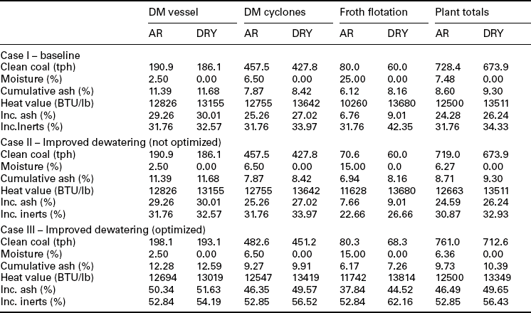
In the next case (Case II), an improved coal dewatering technology was used to reduce the moisture of the flotation product from 25% to 15%. The higher BTU product was accepted and the operating points of the other plant circuits remained unchanged. The lower moisture in the froth flotation circuit reduced the total moisture from 7.48% to 6.27% and increased the heat content from 12 500 to 12 664 BTU/lb (a net improvement of 164 BTU/lb). The net tonnage of saleable coal actually dropped from 728.4 to 719.0 TPH since a smaller amount of moisture reported to clean coal. To optimize performance, the operating points of the cleaning processes were modified such that the same incremental inerts were produced in all circuits (Case III). The lower moisture in the flotation circuit allowed the incremental inerts in all circuits to be raised to over 50% while still maintaining a 12 500 BTU/lb product for the total plant. This modification made it possible to significantly increase both the clean coal ash and tonnage in the dense medium circuits. The ash in the vessel circuit increased from 11.39% to 12.28% and the tonnage increased from 190.9 to 198.1 TPH. Likewise, the ash in the cyclone circuit increased from 7.87% to 9.27% and the tonnage increased from 457.5 to 482.6 TPH. The overall plant moisture decreased from 7.48% to 6.36%. This shift raised the total plant production to 761.0 TPH, which represented an increase of 32.6 TPH as compared to the baseline Case I. This additional tonnage increased the plant production by about 4.4% while still providing a clean coal product at the 12 500 BTU/lb contract specifications. Even if additional penalties were imposed for the higher ash levels, the increased production would still provide sufficient new income to easily pay for the equipment necessary to achieve the moisture reduction.
17.5 Conclusion
The production of clean coal from a preparation plant can be maximized using an optimization principle commonly referred to as the incremental quality concept. This concept dictates that all plant circuits be operated at the same incremental quality to maximize the net value of delivered clean coal product. For efficient processes such as dense medium separators, this constraint can be achieved for all practical purposes by operating all parallel circuits at the same effective RD cutpoint. Less efficient water-based separators, such as spirals and water-only cyclones, require slightly higher cutpoints to correct for the misplacement of particles that tend to lower incremental quality. The amount that the cutpoint must be raised can be estimated from simulation programs that utilize partition models to identify optimal RD cutpoints for each unit operation. In cases where such capabilities are not available on a routine basis, tabular values can be used to approximately estimate optimal cutpoints for each unit operation provided the approximate cleanability of the coal is known. As such, the incremental quality approach to optimization makes it possible to identify optimum operating gravities without conducting detailed analysis of the feed coal washability. The fundamental understanding provided by these practical optimization principles makes it possible for plant operators to effectively improve plant production and to clarify the process of making capital decisions. This strategy is also relatively easy to implement, since RD cutpoints can be readily monitored and controlled by plant operators for optimization purposes.
17.6 Future trends
Coal preparation offers many attractive benefits for coal customers, including lower transportation costs, improved properties for coal utilization, and reduced emissions of particulate and gaseous pollutants. However, the industry must continue to evolve from a technological standpoint so that plants can continue to operate in an increasingly competitive global market. One area in which tremendous strides have been made over the past decade is in the area of plant automation and control (Couch, 1996). The application of on-line sensors, together with programmable logic controllers, has allowed modern plants to operate more efficiently and to respond more quickly to changing market demands. On the other hand, the industry continues to struggle with real-time determination of the quality of coal products (Belbot et al., 2001). Analyzers are commercially available for real-time analysis of many quality parameters for coal, including ash, sulfur, and moisture, although measurement accuracy is often poor because of sampling and calibration issues (Yu et al., 2003). Moreover, analyzers cannot be used to accurately determine important data such as particle size distributions and real-time washability. Therefore, improving automation, control, and sensor technologies is a key challenge for the industry to overcome. If realized in the near future, these advances will enhance the industry’s ability to optimize the production of high-quality coal necessary to maintain profitability.
17.7 References
Abbott, J., The optimisation of process parameters to maximise the profitability from a three-component blend. Proceedings 1st Australian Coal Preparation Conference, 1982:87–105. [6–10 April, Newcastle, Australia].
Abbott, J., Miles, N.J., moothing and interpolation of float-sink data for coals Cornwall, England, Proceedings International Symposium on Gravity Separation. 1990. [12–14 September].
Anonymous. Plotting instantaneous ash versus density. Coal Preparation. 1966; Vol. 2(No. 1):pp. 35.
Armstrong, M., Whitmore, R.L., The mathematical modeling of coal washability. 1st Australia Coal Preparation Conference, 1982:220–239. [6–10 April, Newcastle, Australia].
Belbot, M., Vaurvopoulos, G., Paschal, J., A commercial elemental online coal analyzer using pulsed neutrons. AIP Conference Proceedings. Proceedings CAARI 2000, 16th International Conference on the Application of Accelerators in Research and Industry, 2001:1065–1068. [doi: 10.1063/1.1395489,].
Bethell, P.J., Luttrell, G.H. Effects of ultrafine desliming on coal flotation circuits. Centenary of Flotation Symposium. 2005; Vol. 38:719–728. [Brisbane, Australia, 6–9 June].
Bethell, P.J., Luttrell, G.H., Firth, B., Comparison of preparation plant design practices for metallurgical and stream coal applications. XV International Coal Preparation Conference and Exhibition, 2006:98–110. [Beijing, China, 17–20 October].
Clarkson, C.J., Optimisation of coal production from mine face to customer Makcay, Australia. Proceedings 3rd Large Open Pit Mining Conference, 1992:433–440. [30 August–3 September].
Couch, G., Coal Preparation: Automation and Control. International Energy Agency, London, 1996:64 pp. [IEAPER/22].
Dell, C.C. The Mayer curve. Colliery Guardian. 1956; 33:412–414.
Gupta, V., Mohanty, M.K. Coal preparation plant optimization: a critical review of the existing methods. International Journal of Mineral Processing. 2006; 79(1):9–17.
Kempnich, R., Coal Preparation – A World View Kentucky, USA. Proceedings 17th International Coal Preparation Exhibition and Conference, 2000:5–48. [2–4 May, Lexington].
King, R.P. Practical optimization strategies for coal-washing plants. Coal Preparation. 1999; 20:13–34.
Luckie, P.T., Spicer, T.S., Lovell, H.L., A Method for Determining the Partition Curve of a Coal Washing Process Department of Mineral Preparation. Special Research Report, 1969:318 pp. [Pennsylvania State University].
Luttrell, G.H., Keles, S., Honaker, R.Q., Implications of Constant Incremental Quality on the Design of Fine Coal Dewatering Circuitry 22–25 February 2009. Preprint No 09–093, SME Annual Conference and Exhibit, 2009. [Denver, Colorado].
Luttrell, G.H., Barbee, C.J., Stanley, F.L., Optimum Cutpoints for Heavy Medium Separations Exploration, Inc., Littleton, ColoradoHonaker, R.Q., Forrest, W.R., eds. dvances in Gravity Concentration, 2003:81–91. [Society for Mining, Metallurgy].
Luttrell, G.H., Catarious, D.M., Miller, J.D., Stanley, F.L., An Evaluation of Plantwide Control Strategies for Coal Preparation Plants. Control 2000, 2000:175–184. [SME, Littleton, CO].
Luttrell, G.H., Honaker, R.Q., Bethell, P.J., Stanley, F.L., Design of High-Efficiency Spiral Circuits for Coal Preparation Plants. Designing the Coal Preparation Plant of the Future, 2007:73–87. [SME, Littleton, Colorado].
Mahr, D. Coal blending of power plants. Power Engineering. 1981; 81:86–89.
Mayer, F.W. A new washing curve. Gluckauf. 1950; 86:498–509.
Mohanta, S., Mishra, B.K. On the adequacy of distribution curves used in coal cleaning: a statistical analysis. Fuel. 2009; 88:2262–2268.
Osborne, D.G., Coal Preparation Technology Graham,Trotman, 1988;Vol. 1. [Norwell, Maine 600].
Osborne, D.G., Davis, J.J., Developments in Coal Dewatering in Australia Exploration, Inc., Littleton, Colorado, 1995Dawatra S.K., ed. Chapter 34. High Efficiency Coal Preparation: An International Symposium, 1995:401–408. [Society for Mining, Metallurgy].
Peng, F.F., Luckie, P.T., Process Control, Part 1 – Separation EvaluationLeonard J., Hardinge B., eds. Society of Mining Engineers. 5th Ed. Coal Preparation. Port City Press, Baltimore, Maryland, USA, 1991:659–716.
Rao, B.V., Kapur, P.C., Rahul, K. Modeling the size-density partition surface of dense-medium separators. International Journal of Mineral Processing. 2003; 72(1–4):443–453.
Rayner, J.G. Direct determination of washing parameters to maximize yield at a given ash. Proceedings Australia Institute of Mining and Metallurgy. 1987; 292(8):67–70.
Rong, R.X., Lyman, G.J. Computational techniques for coal washery optimization – parallel gravity and flotation separation. Coal Preparation. 1985; 2:51–67.
Rong, R.X. Optimization of complex coal preparation flowsheets. International Journal of Mineral Processing. 1992; 34(1–2):53–69.
Scott, I.A., Napier-Munn, T.J. Dense-Medium Cyclone Model Based on the Pivot Phenomenon. Trans. Inst. Min. Metall. (Section C: Min. Proc. Extr. Metall.). 1992; Vol. 101:C61–C76.
Tavares, L.M., King, R.P. A useful model for the calculation of the performance of batch and continuous jigs. Coal Preparation. 1995; Vol. 15(No. 3–4):99–128.
Yu, S., Ganguli, R., Walsh, D.E., Bandopadhyay, S., Patil, S.L., Calibration of On-Line Ash Analyzers Using Neural Networks Preprint 03–047. SME Annual Meeting, 2003:4 pp. [24–26 February 2003, Cincinnati, OH].