
12.3 THE IIR FILTER DEPENDENCE GRAPH
We use Eq. 12.1 to study the index dependencies of the algorithm variables. Variable y is an input/output or intermediate variable, and variables x, a, and b are all input variables. An input/output variable is one that is present on the right-hand side (RHS) and left-hand side (LHS) of the algorithm equations with different index dependencies for each side.
We note that the algorithm gives rise to a two-dimensional (2-D) computation domain ![]() since we have two indices, i and j. Since the dimensionality of
since we have two indices, i and j. Since the dimensionality of ![]() is low, it is best to visualize
is low, it is best to visualize ![]() using a dependence graph since this is easier for humans to visualize and analyze.
using a dependence graph since this is easier for humans to visualize and analyze.
We organize our indices in the form of a vector:
(12.2)
![]()
for given values of the indices, the vector corresponds to a point in the ![]() 2 space.
2 space.
12.3.1 The 2-D Dependence Graph
The dimension of a dependence graph is two, which is the number of indices in the algorithm. The graph covers the points p(i, j) ∈ ![]() , where the range of the indices defines the boundaries of the dependence graph as
, where the range of the indices defines the boundaries of the dependence graph as
(12.3)
![]()
Note that ![]() extends to ∞ in the i direction, which defines an extremal ray in that direction.
extends to ∞ in the i direction, which defines an extremal ray in that direction.
The dependence matrices for the variables will help us plot them in the filter dependence graph. We prefer to use the concept of dependence graph here because of the low dimensionality of a dependence graph, which facilitates visualization.
Figure 12.1 shows the dependence graph of the 1-D IIR filter for the case N = 4. The following paragraphs describe how the dependence graph was obtained. The missing circles near the j-axis indicate that there are no operations to be performed at these locations since the input to our filter does not have negative indices.
Figure 12.1 Dependence graph for the 1-D IIR filter for the case N = 4.

The output variable y has a dependence matrix given by
(12.4)
![]()
The null vector associated with this matrix is
(12.5)
![]()
Therefore, the broadcast domains for this variable are vertical lines in ![]() . This is shown in Fig. 12.1 for the case N = 4.
. This is shown in Fig. 12.1 for the case N = 4.
The input variables a and b have a dependence matrix given by
(12.6)
![]()
The null vector associated with this matrix is
(12.7)
![]()
Therefore, the broadcast domains for these two variables are the horizontal lines in ![]() . The input variable x has a dependence matrix given by
. The input variable x has a dependence matrix given by
(12.8)
![]()
The null vector associated with this matrix is
(12.9)
![]()
Therefore, the broadcast domains for this variable are the diagonal lines in ![]() .
.
The input variable y has a dependence matrix given by
(12.10)
![]()
The null vector associated with this matrix is
(12.11)
![]()
Therefore, the broadcast domains for this variable are the diagonal lines in ![]() also.
also.
12.3.2 The Scheduling Function for the 1-D IIR Filter
We start by using an affine scheduling function given by
(12.12)
![]()
where the constant s = 0 since the point at the origin p(0, 0) ∈ ![]() . Any point p = [i j]t ∈
. Any point p = [i j]t ∈ ![]() is associated with the time value
is associated with the time value
(12.13)
![]()
Assigning time values to the nodes of the dependence graph transforms the dependence graph to a directed acyclic graph (DAG) as was discussed in Chapters 10 and 11. More specifically, the DAG can be thought of as a serial–parallel algorithm (SPA) where the parallel tasks could be implemented using a thread pool or parallel processors for software or hardware implementations, respectively. The different stages of the SPA are accomplished using barriers or clocks for software or hardware implementations, respectively.
In order to determine the components of s, we turn our attention to the filter inputs x. The input data are assumed to be supplied to our array at consecutive time steps. From the dependence graph, we see that samples x(i) and x(i + 1) could be supplied at points p1 = [i 0]t and p2 = [i + 1 0]t, respectively. The time steps associated with these two input samples are given from Eq. 10.17 by
(12.14)
![]()
(12.15)
![]()
Assuming that the consecutive inputs arrive at each time step, we have t(p2) − t(p1) = 1, and we must have
(12.16)
![]()
So now we know one component of the scheduling vector based on input data timing requirements. Possible valid scheduling functions could be
(12.17)

All the above timing schedules are valid and have different implications on the timing of the output and partial results. The first scheduling vector results in broadcast input and pipelined output. The second scheduling vector results in broadcast of the output variable y and could produce Design 2, discussed in Chapter 9. The third scheduling vector results in pipelined input and output and could produce Design 3, discussed in Chapter 9. Let us investigate the scheduling vector s = [1 −1]. This choice implies that
(12.18)
![]()
which results in broadcast x and yin samples. Based on our choice for this time function, we obtain the DAG shown in Fig. 12.2. The gray lines indicate equitemporal planes. All nodes lying on the same gray line execute their operations at the time indicated beside the line. The gray numbers indicate the times associated with each equitemporal plane. Notice from the figure that all the input signals x and yin are broadcast to all nodes in an equitemporal plane and output signals yout are pipelined as indicated by the arrows connecting the graph nodes. At this stage, we know the timing of the operations to be performed by each node. We do not know yet which processing element each node is destined to. This is the subject of the next subsection.
Figure 12.2 DAG for the 1-D IIR filter for the case N = 4.

12.3.3 Choice of Projection Direction and Projection Matrix
Chapters 10 and 11 explained that the projection operation assigns a node or a group of nodes in the DAG to a thread or processor. The number of assigned nodes determines the workload associated with each task. The operation also indicates the input and output data involved in the calculations. The projection operation controls the workload assigned to each thread/processor at each stage of the execution of the SPA.
From Chapter 11, a restriction on the projection direction d is that
(12.19)
![]()
Therefore, we have three possible choices for projection directions:
(12.20)
![]()
(12.21)
![]()
(12.22)
![]()
The projection matrices associated with each projection direction are given by
(12.23)
![]()
(12.24)
![]()
(12.25)
![]()
12.3.4 Design 1: Projection Direction d1 = [1 0]t
Since the chosen projection direction is along the extremal ray direction, the number of tasks will be finite. A point p = [i j]t ∈ ![]() maps to the point
maps to the point ![]() , which is given by
, which is given by
(12.26)
![]()
The reduced or projected DAG (![]() ) is shown in Fig. 12.3. Task T(i) stores the two filter coefficients a(i) and b(i). The filter output is obtained from the top tasks and is fed back to the first task at the next time step. Notice that both inputs x and y are pipelined between the tasks.
) is shown in Fig. 12.3. Task T(i) stores the two filter coefficients a(i) and b(i). The filter output is obtained from the top tasks and is fed back to the first task at the next time step. Notice that both inputs x and y are pipelined between the tasks.
Figure 12.3 ![]() for the 1-D IIR filter for the case N = 4 and d1 = [1 0]t. (a) The
for the 1-D IIR filter for the case N = 4 and d1 = [1 0]t. (a) The ![]() for the tasks. (b) Task processing details and array implementation.
for the tasks. (b) Task processing details and array implementation.

12.3.5 Design 2: Projection Direction d2 = [0 1]t
A point p = [i j]t ∈ ![]() maps to the point
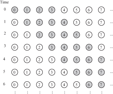
maps to the point ![]() = i. The pipeline is shown in Fig. 12.4. Each task stores all the filter coefficients and is responsible for producing an output sample, which reduces intertask communication requirements. Task T(i) accepts input samples x(i − N + 1) to x(i) from the memory or input data bus at time steps i − N + 1 to i. Task T(i) also reads the memory or the output data bus for samples yin(i − N + 1) to yin(i − 1) at time steps i − N + 1 to i − 1. Task T(i) produces the output yout(i) at time step i and stores that signal in the shared memory or places the signal on the output data bus for the case of hardware implementation. The number of tasks is infinite since our projection direction did not coincide with the ray direction. However, each task is active for the duration of N time steps. The task activities at different time steps are shown in Fig. 12.5. The timing diagram thus indicates that we could merge the tasks. Therefore, we relabel the task indices such that T(i) maps to T(j), such that
= i. The pipeline is shown in Fig. 12.4. Each task stores all the filter coefficients and is responsible for producing an output sample, which reduces intertask communication requirements. Task T(i) accepts input samples x(i − N + 1) to x(i) from the memory or input data bus at time steps i − N + 1 to i. Task T(i) also reads the memory or the output data bus for samples yin(i − N + 1) to yin(i − 1) at time steps i − N + 1 to i − 1. Task T(i) produces the output yout(i) at time step i and stores that signal in the shared memory or places the signal on the output data bus for the case of hardware implementation. The number of tasks is infinite since our projection direction did not coincide with the ray direction. However, each task is active for the duration of N time steps. The task activities at different time steps are shown in Fig. 12.5. The timing diagram thus indicates that we could merge the tasks. Therefore, we relabel the task indices such that T(i) maps to T(j), such that
(12.27)
![]()
Figure 12.4 ![]() for the 1-D IIR filter for the case N = 4 and d2 = [0 1]t.
for the 1-D IIR filter for the case N = 4 and d2 = [0 1]t.

Figure 12.5 Task activities for the 1-D FIR filter for the case N = 4 and d2 = [0 1]t.
The reduced DAG is shown is in Fig. 12.6.
Figure 12.6 The reduced ![]() for the 1-D FIR filter for N = 4 and d2 = [0 1]t. (a) The
for the 1-D FIR filter for N = 4 and d2 = [0 1]t. (a) The ![]() (b) Task processing details.
(b) Task processing details.
