21.2 FDM FOR 1-D SYSTEMS

We start by explaining how FDM is applied to a 1-D system for simplicity. Assume the differential equation describing our system is second order of the form

(21.8)

Note that we normalized the length such that the maximum value of x is 1. The associated boundary conditions are given by

(21.9)

(21.10)

(21.11)

where v₀ describes the value of the variable at x = 0, v₁ describes the value of the variable at x = 1, and f(x) describes the initial values of the variable. Note that the boundary conditions at x = 0 and x = 1 might, in the general case, depend on time as v₀(t) and v₁(t). Usually, a is a simple constant. In the general case, a might depend both on time and space as a(x, t).

It might prove difficult to solve the system described by Eq. 21.8 when the boundary conditions are time dependent or the medium is inhomogeneous and/or time dependent. To convert the system equation to partial difference equation, we need to approximate the derivatives v_x and v_xx. Using Taylor series, we can describe the first derivative as

(21.12)

(21.13)

where Δx is the grid size. The value of Δx is determined by the number of grid points I:

(21.14)

From these two expressions, we can express v_x in the central difference formula:

(21.15)

Likewise, we can obtain v_xx and v_tt using the formulas

(21.16)

(21.17)

The value of Δt is determined by the number of time iterations K and assuming that the total simulation time is 1:

(21.18)

Our choice of Δx and Δt divides the x-t plane into rectangles of sides Δx and Δt. A point (x, t) in the x-t plane can be expressed in terms of two indices i and k:

(21.19)

(21.20)

Using the indices i and k, we can rewrite Eqs. 21.16 and 21.17 in the simpler form:

(21.21)

(21.22)

Combining Eqs. 21.8, 21.21, and 21.22, we finally can write

(21.23)

with

(21.24)

Thus, we are able to compute v(i, k + 1) at time k + 1 knowing the values of v at times k and k − 1.

Equation 21.23 describes a 2-D regular iterative algorithm (RIA) in the indices i and k. Figure 21.1 shows the dependence graph for the 1-D finite difference algorithm for the case I = 10 and K = 15. Figure 21.1a shows how node at position (4,8) depends on the data from nodes at points (3,7), (4,7), (4,6), and (5,7). Figure 21.1b shows the complete dependence graph.

Figure 21.1 Dependence graph for the 1-D finite difference algorithm for the case I = 10 and K = 15. (a) Showing the dependence of the node at the black circle on the data from the gray circles. (b) The complete dependence graph.

21.2.1 The Scheduling Function for 1-D FDM

Since the dependence graph of Fig. 21.1b is 2-D, we can simply use the results of Chapter 10. Our scheduling function is specified as

(21.25)

(21.26)

Assigning time values to the nodes of the dependence graph transforms the dependence graph to a directed acyclic graph (DAG) as was discussed in Chapters 10 and 11. More specifically, the DAG can be thought of as a serial–parallel algorithm (SPA) where the parallel tasks could be implemented using a thread pool or parallel processors for software or hardware implementations, respectively. The different stages of the SPA are accomplished using barriers or clocks for software or hardware implementations, respectively.

We have several restrictions on t(p) according to the data dependences depicted in Fig. 21.1:

(21.27)

From the above restrictions, we can have three possible simple timing functions that satisfy the restrictions:

(21.28)

(21.29)

(21.30)

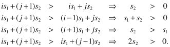
Figure 21.2 shows the DAG for the three possible scheduling functions for the 1-D FDM algorithm when I = 5 and K = 9. For s₁, the work (W) to be done by the parallel computing system is equal to I + 1 calculations per iteration. The time required to complete the problem is K + 1.

Figure 21.2 Directed acyclic graphs (DAG) for the three possible scheduling functions for the 1-D FDM algorithm when I = 5 and K = 9.

For s₂ and s₃, the work (W) to be done by the parallel computing system is equal to [I/2] calculations per iteration. The time required to complete the problem is given by I + 2K.

Linear scheduling does not give us much control over how much work is to be done at each time step. As before, we are able to control the work W by using nonlinear scheduling functions of the form given by

(21.31)

where n is the level of data aggregation.

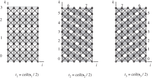
Figure 21.3 shows the DAG for the three possible nonlinear scheduling functions for the 1-D FDM algorithm when I = 5, K = 9, and n = 3. For nonlinear scheduling based on s₁, the work (W) to be done by the parallel computing system is equal to n(I + 1) calculations per iteration. The time required to complete the problem is |K/n|. For nonlinear scheduling based on s₂ and s₃, the work (W) to be done by the parallel computing system is equal to K calculations per iteration. The time required to complete the problem is given by |(I + 2K)/n|.

Figure 21.3 Directed acyclic graphs (DAG) for the three possible nonlinear scheduling functions for the 1-D FDM algorithm when I = 5, K = 9, and n = 3.

21.2.2 Projection Directions

The combination of node scheduling and node projection will result in determination of the work done by each task at any given time step. The natural projection direction associated with s₁ is given by

(21.32)

In that case, we will have I + 1 tasks. At time step k + 1, task T_i is required to perform the operations in Eq. 21.23. Therefore, there is necessary communication between tasks T_i, T_{i − 1}, and T_{i − 1}. The number of messages that need to be exchanged between the tasks per time step is 2I.

We will pick projection direction associated with s₂ or s₃ as

(21.33)

In that case, we will have I + 1 tasks. However, the even tasks operate on the even time steps and the odd tasks operate on the odd time steps. We can merge the adjacent even and odd tasks and we would have a total of [(I + 1)/2] tasks operating every clock cycle. There is necessary communication between tasks T_i, T_i−1, and T_i−1. The number of messages that need to be exchanged between the tasks per time step is 3[(I − 2)/2] + 4.

Linear projection does not give us much control over how much work is assigned to each task per time step or how many messages are exchanged between the tasks. We are able to control the work per task and the total number of messages exchanged by using nonlinear projection operation of the form

(21.34)

where P is the projection matrix associated with the projection direction and m is the number of nodes in the DAG that will be allocated to a single task. The total number of task depends on I and m and is given approximately by 3[I/m].