2.5 PIPELINING

Pipelining is a very effective technique for improving system throughput, which is defined as the rate of task completion per unit time. This technique requires two conditions to be effective:

An often quoted example of successful pipelining is car manufacture. We note that this satisfies the two requirements of pipelining: we have many cars to manufacture and the manufacture of each car requires manufacture of several components.

A pipeline executes a task in successive stages by breaking it up into smaller tasks. It is safe to assume that a smaller task will be completed in a shorter time compared to the original task. As explained above, the idea of a pipeline is to execute a serial task using successive pipeline stages and placing registers between the stages to store the intermediate results.

2.5.1 Estimating Pipeline Speed

Figure 2.10 shows a general organization of a pipeline where the C/L blocks indicate combinational logic blocks composed of logic gates. The Reg blocks indicate edge-triggered registers to store intermediate results. The speed of that pipeline depends on the largest combinational logic delay of the C/L blocks. Figure 2.11 shows how the clock speed of the pipeline is calculated. The figure illustrates several delays:

Figure 2.10 General structure for pipeline processing.

Figure 2.11 Estimating clock speed for a pipeline based on pipeline delays. (a) One stage of a pipeline. (b) Signal delays due to the registers and combinational logic blocks.

The formula for estimating the clock frequency is given by

(2.9)

(2.10)

where T_C/L,max is the maximum delay of the combinational logic blocks, τ_skew is the maximum expected clock skew between adjacent registers, and τ_setup is the setup time for a register.

A classic example of pipelining is in the way a computer executes instructions. A computer instruction goes through four steps:

The above steps are dependent and must be executed serially in the order indicated above. We cannot reverse the order or even do these steps in parallel (i.e., simultaneously). So, without pipelining, the processor would need three clock cycles per instruction. We can see that processing computer instructions satisfies the pipeline requirements: we have several instructions and each instruction is divisible into several serial subtasks or stages.

A serial implementation of the above tasks is shown in Fig. 2.12. We see that the fetch operation of the next instruction can only start after all the opera­tions associated with the current instruction are completed. Now we can show a sketch of a pipeline to process computer instructions as shown in Fig. 2.13. Instruction processing could be looked at in more detail than implied by the above processing stages. A nice discussion of the instruction cycle can be found in Reference 18.

Figure 2.12 Time needed for the serial processing of a computer instruction.

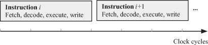
Figure 2.13 Instruction pipeline processing.

Now let us see how this pipeline can speed up the instruction processing. Figure 2.14 shows the instruction pipeline during program execution. Each row in the figure shows the activities of each processing stage during the successive clock cycles. So, the first row shows the contents of the IR after each fetch operation. The second row shows the instructions being decoded at the different clock cycles. The third row shows the instructions being executed by the ALU during each clock cycle as well as storing the result in a register. If we trace each instruction through the pipeline stages, we conclude that each instruction requires three clock cycles to be processed. However, we also note that each hardware unit is active during each clock cycle as compared to Fig. 2.12. Therefore, the pipeline executes an instruction at each clock cycle, which is a factor of three better than serial processing. In general, when the pipeline is running with data in every pipeline stage, we expect to process one instruction every clock cycle. Therefore, the maximum speedup of a pipeline is n, where n is the number of pipeline stages.

Figure 2.14 Pipeline processing of computer instructions during program execution.

There is one problem associated with using pipelining for processing computer instructions. Conditional branching alters the sequence of instructions that need to be executed. However, it is hard to predict the branching when the instructions are being executed in sequence by the pipeline. If the sequence of the instructions needs to be changed, the pipeline contents must be flushed out and a new sequence must be fed into the pipeline. The pipeline latency will result in the slowing down of the instruction execution.

Now we turn our attention to showing how pipelining can increase the throughput of the ALU/datapath. We use this topic to distinguish between pipelining and parallel processing. We can use the example of the inner product operation often used in many digital signal processing applications. Inner product operation involves multiplying several pairs of input vectors and adding the results using an accumulator:

(2.11)

As mentioned before, the above operation is encountered in almost all digital signal processing algorithms. For example, the finite impulse response (FIR) digital filter algorithm given by the following equation is an example of an inner product operation (sure, it is convolution, but we are assuming here the shifted samples are stored as a vector!):

(2.12)

We can iteratively express evaluation of y(i) in the form

(2.13)

The operation in Eq. 2.13 is often referred to as the multiply/accumulate (MAC) operation. Again, this operation is so important in digital signal processing that there are special MAC instructions and hardware to implement it. The FIR algorithm satisfies pipelining requirements: we have several tasks to be completed, which are the repeated MAC operations. Also, each MAC operation can be broken down into two serial subtasks: the multiply followed by the add operations.

Figure 2.15 shows how we can implement each MAC iterative step using parallel or pipelined hardware. In this diagram, we assumed that we are using a parallel multiplier to effect the multiplication operation. The parallel implementation of Fig. 2.15a shows that the multiply and add operations are done in the same clock cycle and the adder output is used to update the contents of the accumulator. The clock period or time delay for these two operations is given by

(2.14)

Figure 2.15 Multiply/accumulate (MAC) implementation options. (a) Parallel implementation. (b) Pipelined implementation.

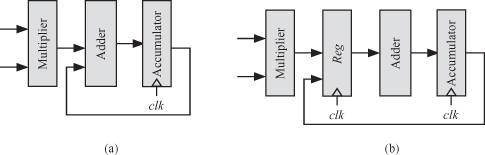
Assuming that the parallel multiplier delay is double the adder delay, the above equation becomes

(2.15)

Now consider the pipelined MAC implementation Fig. 2.15b. The output of the multiplier is stored in a register before it is fed to the adder. In that case, the clock period is determined by the slowest pipeline stage. That stage is the multiplier and our clock period would be given by

(2.16)

In effect, the pipelined design is approximately 30% faster than the parallel design. We should point out before we leave this section that many hardware design innovations are possible to obtain much better designs than those reported here. The interested reader could refer to the literature such as References 21–23.