9.5 DESIGN 1: USING HORNER’S RULE FOR BROADCAST INPUT AND PIPELINED OUTPUT
Suppose we want to evaluate the polynomial for a certain value of x:
(9.8)
![]()
We can rewrite the polynomial using Horner’s scheme as
(9.9)
![]()
Now the polynomial is recursively evaluated through the following steps:
1. Evaluate the innermost term y0 = 2x + 4.
2. Evaluate the next innermost term y1 = y0 x + 5.
3. Evaluate the term y2 = y1x + 3.
4. Evaluate the term y3 = y2x + 9.
5. Evaluate p(x) to y3.
Now we apply Horner’s’ scheme to Eq. 9.7 to obtain the recursive expression
(9.10)
![]()
The above equation can be written as
(9.12)
![]()
(9.13)
![]()
(9.14)
![]()
Based on the above iterative expression, task T (i) computes Yi in Eq. 9.11 using one multiplication and one addition:
(9.15)
![]()
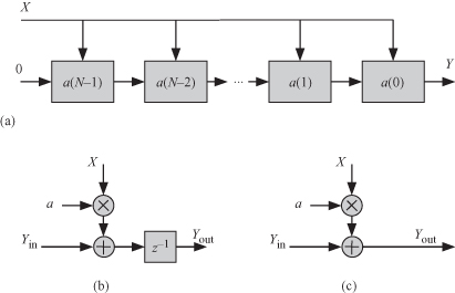
The output of T(i) is saved then forwarded to T(i − 1) and the input to T(N − 1) is initialized to 0. Figure 9.2a shows the resulting directed acyclic graph (DAG) for an output sample, y. The figure can be replicated to show the different DAGs for other output samples. When these tasks are implemented in hardware, this DAG becomes the systolic array structure that implements the FIR filter. This structure is actually one of the classical canonic realizations of Eq. 9.7. Figure 9.2b shows the details of a processor element in case of hardware implementation of the DAG. Note that the input signal is broadcast to all tasks and the output is pipelined between the tasks.
Figure 9.2 FIR digital filter software/hardware implementation with pipelined outputs. (a) DAG for FIR digital filter. (b) Processor element details.