
10.8 SOFTWARE AND HARDWARE IMPLEMENTATIONS OF THE DAG TECHNIQUE
By using different scheduling functions and projection directions, the DAG is converted to a set of tasks that can be executed concurrently in software threads or in hardware systolic arrays. The technique maps the DAG of the algorithm to simultaneous multithreaded (SMT) tasks or single instruction multiple data stream (SIMD)/systolic hardware. In the following section, we shall refer to the computations at each node as tasks, knowing that tasks translate to threads in software or PEs in hardware. In all cases discussed in this section we choose the scheduling function s = [1 –1].
10.8.1 Design 1: Projection Direction d1 = [1 0]t
Since the chosen projection direction is along the extremal ray direction, the number of concurrent tasks will be finite. A point p = [i j]t ∈ DAG maps to the point ![]() . The pipeline is shown in Fig. 10.5. Task T(i) stores the filter coefficient a(i). The filter output is obtained from the rightmost PE. Notice that both inputs x and y are pipelined between the PEs. Some explanation of notation in the
. The pipeline is shown in Fig. 10.5. Task T(i) stores the filter coefficient a(i). The filter output is obtained from the rightmost PE. Notice that both inputs x and y are pipelined between the PEs. Some explanation of notation in the ![]() is in order. An arrow connecting tasks T(i) to task T(j) indicates that the output data of T(i) is stored in memory and is made available to T(j) at the next time step. An arrow exiting a task indicates calculations or data to be completed by the task at the end of the time step. An arrow entering a task indicates data read at the start of the time step.
is in order. An arrow connecting tasks T(i) to task T(j) indicates that the output data of T(i) is stored in memory and is made available to T(j) at the next time step. An arrow exiting a task indicates calculations or data to be completed by the task at the end of the time step. An arrow entering a task indicates data read at the start of the time step.
Figure 10.5 Projected DAG (![]() ) for the 1-D FIR filter for the case N = 4, s = [1 –1], and d1 = [1 0]t. (a) The resulting
) for the 1-D FIR filter for the case N = 4, s = [1 –1], and d1 = [1 0]t. (a) The resulting ![]() . (b) The task processing details.
. (b) The task processing details.

10.8.2 Design 2: Projection Direction d2 = [0 −1]t
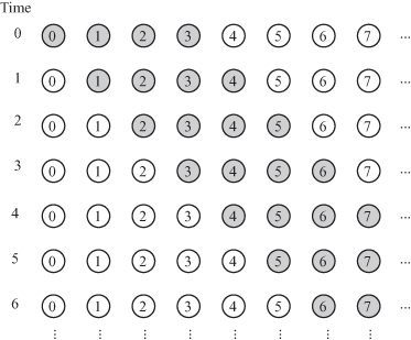
A point p = [i j]t ∈ D maps to the point ![]() . The pipeline is shown in Fig. 10.6. Each task stores all the filter coefficients locally to reduce intertask communication requirements. T(i) accepts input samples x(i − N + 1) to x(i) from the shared memory or input data bus at time step i. T(i) produces the output yout(i) at time step i and stores that data in memory or sends that signal onto the output data bus. The number of tasks is infinite since our projection direction did not coincide with the ray direction. However, each task is active for the duration of N time steps. The task activities at different time steps are shown in Fig. 10.7. The timing diagram thus indicates that we could merge the tasks. Therefore, we relabel the task indices such that T(i) maps to T(j), such that
. The pipeline is shown in Fig. 10.6. Each task stores all the filter coefficients locally to reduce intertask communication requirements. T(i) accepts input samples x(i − N + 1) to x(i) from the shared memory or input data bus at time step i. T(i) produces the output yout(i) at time step i and stores that data in memory or sends that signal onto the output data bus. The number of tasks is infinite since our projection direction did not coincide with the ray direction. However, each task is active for the duration of N time steps. The task activities at different time steps are shown in Fig. 10.7. The timing diagram thus indicates that we could merge the tasks. Therefore, we relabel the task indices such that T(i) maps to T(j), such that
(10.52)
![]()
Figure 10.6 Projected DAG (![]() ) for the 1-D FIR filter for the case N = 4, s = [1 –1], and d2 = [0 –1]t.
) for the 1-D FIR filter for the case N = 4, s = [1 –1], and d2 = [0 –1]t.
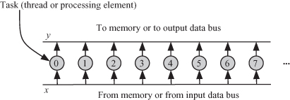
Figure 10.7 Task activity for the 1-D FIR filter for the case N = 4, s = [1 –1], and d2 = [0 –1]t.
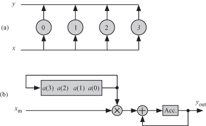
The reduced ![]() is shown in Fig. 10.8.
is shown in Fig. 10.8.
Figure 10.8 The reduced ![]() for the 1-D FIR filter for N = 4, s = [1 –1], and d2 = [0 –1]t. (a) The
for the 1-D FIR filter for N = 4, s = [1 –1], and d2 = [0 –1]t. (a) The ![]() . (b) The task processing details.
. (b) The task processing details.
10.9 PROBLEMS
10.1. Given are two causal signals h(n) and x(n), which are N samples each. Their cross-correlation is given by the equation
![]()
where n = 0, 1, … , N − 1. Assuming N = 5:
(1) Draw the dependence graph for the algorithm where the index n is to be drawn on the horizontal axis and the index k is to be drawn on the vertical axis.
(2) Write down nullvectors and basis vectors for the algorithm variables.
(3) Find possible simple scheduling functions for this algorithm and discuss the implication of each function on the pipelining and broadcasting of the variables.
(4) Choose one scheduling function and draw the associated DAG for the algorithm.
(5) Show possible nonlinear scheduling options for the scheduling function you chose in part 4.
(6) Find possible projection directions corresponding to the scheduling function you chose in part 4.
(7)
Choose one projection direction and draw the resulting ![]() and the PE details for systolic array implementation.
and the PE details for systolic array implementation.
(8) Show possible nonlinear projection options for the projection direction you chose in part 7.
10.2. The autocorrelation is obtained when, in the problem, we replace signal h(n) with x(n). Study the problem for this situation.
10.3. Apply the dependence graph technique to the sparse matrix–vector multiplication algorithm.
10.4. Apply the dependence graph technique to the sparse matrix–matrix multiplication algorithm.
10.5. Draw the dependence graph of the discrete Hilber transform (DHT) and design multithreaded and systolic processor structures.
10.6. Draw the dependence graph of the inverse discrete Hilber transform (IDHT) and design multithreaded and systolic processor structures.