
1.8 MEASURING BENEFITS OF PARALLEL COMPUTING
We review in this section some of the important results and benefits of using parallel computing. But first, we identify some of the key parameters that we will be studying in this section.
1.8.1 Speedup Factor
The potential benefit of parallel computing is typically measured by the time it takes to complete a task on a single processor versus the time it takes to complete the same task on N parallel processors. The speedup S(N) due to the use of N parallel processors is defined by
(1.6)
![]()
where Tp(1) is the algorithm processing time on a single processor and Tp(N) is the processing time on the parallel processors. In an ideal situation, for a fully parallelizable algorithm, and when the communication time between processors and memory is neglected, we have Tp (N) = Tp (1)/N, and the above equation gives
It is rare indeed to get this linear increase in computation domain due to several factors, as we shall see in the book.
1.8.2 Communication Overhead
For single and parallel computing systems, there is always the need to read data from memory and to write back the results of the computations. Communication with the memory takes time due to the speed mismatch between the processor and the memory [14]. Moreover, for parallel computing systems, there is the need for communication between the processors to exchange data. Such exchange of data involves transferring data or messages across the interconnection network.
Communication between processors is fraught with several problems:
1. Interconnection network delay. Transmitting data across the interconnection network suffers from bit propagation delay, message/data transmission delay, and queuing delay within the network. These factors depend on the network topology, the size of the data being sent, the speed of operation of the network, and so on.
2. Memory bandwidth. No matter how large the memory capacity is, access to memory contents is done using a single port that moves one word in or out of the memory at any give memory access cycle.
3. Memory collisions, where two or more processors attempt to access the same memory module. Arbitration must be provided to allow one processor to access the memory at any given time.
4. Memory wall. The speed of data transfer to and from the memory is much slower than processing speed. This problem is being solved using memory hierarchy such as
![]()
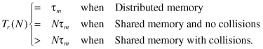
To process an algorithm on a parallel processor system, we have several delays as explained in Table 1.1.
Table 1.1 Delays Involved in Evaluating an Algorithm on a Parallel Processor System
| Operation | Symbol | Comment |
| Memory read | Tr (N) | Read data from memory shared by N processors |
| Memory write | Tw (N) | Write data from memory shared by N processors |
| Communicate | Tc (N) | Communication delay between a pair of processors when there are N processors in the system |
| Process data | Tp (N) | Delay to process the algorithm using N parallel processors |
1.8.3 Estimating Speedup Factor and Communication Overhead
Let us assume we have a parallel algorithm consisting of N independent tasks that can be executed either on a single processor or on N processors. Under these ideal circumstances, data travel between the processors and the memory, and there is no interprocessor communication due to the task independence. We can write under ideal circumstances
(1.8)
![]()
(1.9)
![]()
The time needed to read the algorithm input data by a single processor is given by
(1.10)
![]()
where τm is memory access time to read one block of data. We assumed in the above equation that each task requires one block of input data and N tasks require to read N blocks. The time needed by the parallel processors to read data from memory is estimated as
(1.11)
![]()
where α is a factor that takes into account limitations of accessing the shared memory. α = 1/N when each processor maintains its own copy of the required data. α = 1 when data are distributed to each task in order from a central memory. In the worst case, we could have α > N when all processors request data and collide with each other. We could write the above observations as
(1.12)
Writing back the results to the memory, also, might involve memory collisions when the processor attempts to access the same memory module.
(1.13)
![]()
(1.14)
![]()
For a single processor, the total time to complete a task, including memory access overhead, is given by
(1.15)
![]()
Now let us consider the speedup factor when communication overhead is considered:
(1.16)
![]()
The speedup factor is given by
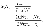
Define the memory mismatch ratio (R) as
(1.18)
![]()
which is the ratio of the delay for accessing one data block from the memory relative to the delay for processing one block of data. In that sense, τp is expected to be orders of magnitude smaller than τm depending on the granularity of the subtask being processed and the speed of the memory.
We can write Eq. 1.17 as a function of N and R in the form
(1.19)
![]()
Figure 1.7 shows the effect of the two parameters, N and R, on the speedup when α = 1. Numerical simulations indicated that changes in α are not as significant as the values of R and N. From the above equation, we get full speedup when the product RN ![]() 1. This speedup is similar to Eq. 1.7 where communication overhead was neglected.
1. This speedup is similar to Eq. 1.7 where communication overhead was neglected.
Figure 1.7 Effect of the two parameters, N and R, on the speedup when α = 1.
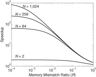
This situation occurs in the case of trivially parallel algorithms as will be discussed in Chapter 7.
Notice from the figure that speedup quickly decreases when RN > 0.1. When R = 1, we get a communication-bound problem and the benefits of parallelism quickly vanish. This reinforces the point that memory design and communication between processors or threads are very important factors. We will also see that multicore processors, discussed in Chapter 3, contain all the processors on the same chip. This has the advantage that communication occurs at a much higher speed compared with multiprocessors, where communication takes place across chips. Therefore, Tm is reduced by orders of magnitude for multicore systems, and this should give them the added advantage of small R values.
The interprocessor communication overhead involves reading and writing data into memory:
(1.20)
![]()
where β ≥ 0 and depends on the algorithm and how the memory is organized. β = 0 for a single processor, where there is no data exchange or when the processors in a multiprocessor system do not communicate while evaluating the algorithm. In other algorithms, β could be equal to log2 N or even N. This could be the case when the parallel algorithm programmer or hardware designer did not consider fully the cost of interprocessor or interthread communications.