15.6 DESIGN 1: DESIGN SPACE EXPLORATION WHEN s = [1 1]^t

The feeding point of input sample t₀ is easily determined from Fig. 15.1 to be p = [0 0]^t. The time value associated with this point is t(p) = 0. Using Eq. 15.3, we get s = 0. Applying the scheduling function in Eq. 15.8 to e_P and e_T, we get

(15.13)

(15.14)

This choice for the timing function implies that both input variables P and Y will be pipelined. The pipeline direction for the input T flows in a southeast direction in Fig. 15.1. The pipeline for T is initialized from the top row in the figure defined by the line j = m − 1. Thus, the feeding point of t₀ is located at the point p = [−m m]^t. The time value associated with this point is given by

(15.15)

Thus, the scalar s should be s = −2m. The tasks at each stage of the SPA derived in this section will have a latency of 2m time steps compared to Design 1.a.

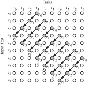
Figure 15.2 shows how the dependence graph of Fig. 15.1 is transformed to the DAG associated with s = [1 1]^t. The equitemporal planes are shown by the gray lines and the execution order is indicated by the gray numbers. We note that the variables P and Y are pipelined between tasks, while variable T is broadcast among tasks lying in the same equitemporal planes. Pipelining means that a value produced by a source task at the end of a time step is used by a destination task at the start of the next time step. Broadcasting means that a value is made available to all tasks at the start of a time step.

Figure 15.2 DAG for Design 1 when n = 10 and m = 4.

There are three simple projection vectors such that all of them satisfy Eq. 15.12 for the scheduling function in Eq. 15.8.

The three projection vectors will produce three designs:

(15.16)

(15.17)

(15.18)

The corresponding projection matrices could be given by

(15.19)

(15.20)

(15.21)

Our task design space now allows for three configurations for each projection vector for the chosen timing function. In the following sections, we study the multithreaded implementations associated with each design option.

15.6.1 Design 1.a: Using s = [1 1]^t and d_a = [1 0]^t

A point in the DAG given by the coordinate p = [i j]^t will be mapped by the projection matrix P_a into the point

(15.22)

A corresponding to Design 1.a is shown in Fig. 15.3. Input T is broadcast to all nodes or tasks in the graph and word p_j of the pattern P is allocated to task T_j. The intermediate output of each task is pipelined to the next task with a higher index such that the output sample y_i is obtained from the rightmost task T_m−1. consists of m tasks and each task is active for n time steps.

Figure 15.3 for Design 1.a when m = 4.

15.6.2 Design 1.b: Using s = [1 1]^t and d_b = [0 1]^t

A point in the DAG given by the coordinate p = [i j]^t will be mapped by the projection matrix P_b into the point

(15.23)

The projected is shown in Fig. 15.4. consists of n − m + 1 tasks. Word p_i of the pattern P is fed to task T₀ and from there, it is pipelined to the other tasks. The text words t_i are broadcast to all tasks. Output y_i is obtained from task t_i at time step i and is broadcast to other tasks. Each task is active for m time steps only. Thus, the tasks are not well utilized as in Design 1.a. However, we note from the DAG of Fig. 15.4 that task T₀ is active for the time step 0 to m − 1, and T_m is active for the time period m to 2m − 1. Thus, these two tasks could be mapped to a single task without causing any timing conflicts. In fact, all tasks whose index is expressed as

(15.24)

Figure 15.4 for Design 1.b when n = 10 and m = 4.

can all be mapped to the same node without any timing conflicts. The resulting after applying the above modulo operations on the array in Fig. 15.4 is shown in Fig. 15.5. The now consists of m tasks. The pattern P could be chosen to be stored in each task or it could circulate among the tasks where initially T_i stores the pattern word p_i. We prefer the former option since memory is cheap, while communications between tasks will always be expensive in terms of area, power, and delay. The text word t_i is broadcast on the input bus to all tasks. T_i produces outputs i, i + m, i + 2m, … at times i, i + m, i + 2m, and so on.

Figure 15.5 Reduced for Design 1.b when n = 10 and m = 4.

15.6.3 Design 1.c: Using s = [1 1]^t and d_c = [1 1]^t

A point in the DAG given by the coordinate p = [i j]^t will be mapped by the projection matrix P_c into the point

(15.25)

The resulting tasks are shown in Fig. 15.6 for the case when n = 10 and m = 4, after adding a fixed increment to all task indices to ensure nonnegative task index values. The DAG consists of n tasks where only m of the tasks are active at a given time step as shown in Fig. 15.7. At time step i, input text t_i is broadcast to all tasks in DAG. We notice from Fig. 15.7 that at any time step, only m out of the n tasks are active. To improve task utilization, we need to reduce the number of tasks. An obvious task allocation scheme could be derived from Fig. 15.7. In that scheme, operations involving the pattern word p_i are allocated to task T_i. In that case, the DAG in Fig. 15.3 will result.

Figure 15.6 Tasks at each SPA stage for Design 1.c.

Figure 15.7 Task activity at the different time steps for Design 1.c.