8.4 FORMAL TECHNIQUE FOR ANALYZING NSPAs

In this chapter, we will show that representing an algorithm by a DG is suitable only when the number of tasks comprising the algorithm is small. However, it is difficult to extract some of the algorithm properties from an inspection of the graph.

For example, it is simple to find W by counting the number of nodes in the graph. Estimating D is slightly more difficult since it involves path search, while estimating P is even more difficult by inspecting the graph.

We need to introduce a more formal technique to deal with the case when the number of tasks is large or when we want to automate the process of extracting the algorithm W, D, and P parameters. We will refer to the tasks of the algorithm as nodes since that was the term we used in the DG description. The technique we explain here converts the DAG of an NSPA into a DAG for an SPA.

Given W nodes/tasks, we define the 0-1 adjacency matrix A, which is a square W × W matrix defined so that element a(i, j) = 1 indicates that node i depends on node j. The source node is j and the destination node is i. Of course, we must have a(i, i) = 0 for all values of 0 ≤ i < W since node i does not depend on itself (self-loop) and we assumed that we do not have any loops. As an example, the adjacency matrix for the algorithm in Fig. 8.1 is given by

(8.2)

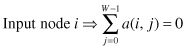
Matrix A has some interesting properties related to our topic. An input node i is associated with row i, whose elements are all zeros. An output node j is associated with column j, whose elements are all zeros. We can write

(8.3)

(8.4)

All other nodes are interior nodes. Note that all the elements in rows 0, 1, and 2 are all zeros since nodes 0, 1, and 2 are input nodes. This is indicated by the bold entries in these three rows. Note also that all elements in columns 7 and 9 are all zeros since nodes 7 and 9 are output nodes. This is indicated by the bold entries in these two columns. All other rows and columns have one or more nonzero elements to indicate interior nodes. If node i has element a(i, j) = 1, then we say that node j is a parent of node i.

From the DAG, we get the following adjacency matrix:

8.4.1 Significance of Powers of Aⁱ: The Connectivity Matrix

Let us see what happens if we raise the adjacency matrix in (8.2) to a higher power. We square the matrix to get matrix A₂ defined as the adjacency matrix raised to the power 2.

(8.5)

There are few nonzero entries and some entries are not 1 anymore. Element a₂ (7, 0) is 1 to indicate that there is a two-hop path from node 0 to node 7. We call A₂ the connectivity matrix of degree 2 to indicate that it shows all two-hop connections between nodes in the graph. Specifically, that path is 0 → 3 → 7. Node 7 has another two-hop path as indicated by element a₂ (7, 1), which is path 1 → 4 → 7. Element a₂ (9, 2) = 2, which indicates that there are two alternative two-hop paths to node 9 starting at node 2. These two paths are 2 → 5 → 9 and 2 → 6 → 9.

Now let us look at the connectivity matrix of order 3, that is, A³:

(8.6)

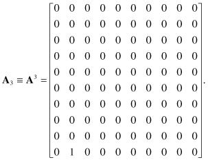
Now all the elements of A³ are zero except for a₃ (9, 1). This indicates that there is only one three-hop path between nodes 1 and 9, specifically, 1 → 4 → 8 → 9. Let us now go one step further and see the value of A⁴:

(8.7)

The fact that all elements of A₄ are zero indicates that there are no paths with a length of four hops. Of course, this implies that all powers of Aⁱ for i > 3 will be zero also. Thus, we can determine the critical path or paths from the highest power of A for which the result is not the zero matrix.