15.8 DESIGN 3: DESIGN SPACE EXPLORATION WHEN s = [1 0]^t

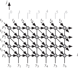
The dependence graph of Fig. 15.1 is transformed to the DAG in Fig. 15.11, which is associated with s = [1 0]^t. The equitemporal planes are shown by the gray lines and the execution order is indicated by the gray numbers. We note that the variables P and T are pipelined between tasks, while variable Y is broadcast among tasks lying in the same equitemporal planes.

Figure 15.11 DAG for Design 3 when n = 10 and m = 4.

There are three simple projection vectors such that all of them satisfy Eq. 15.12 for the scheduling function. The three projection vectors are

(15.29)

(15.30)

(15.31)

Our multithreading design space now allows for three configurations for each projection vector for the chosen timing function.

15.8.1 Design 3.a: Using s = [1 0]^t and d_a = [1 0]^t

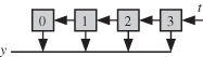
The corresponding to Design 3.a is drawn in Fig. 15.12 for the case when n = 10 and m = 4. Task T_j stores only the value p_j, which can be stored in a register similar to Design 1.a. The outputs of all the tasks must be combined using a reduce operation.

Figure 15.12 for Design 3.a.

These two projection vectors produce the same configuration as Design 3.a. However, unlike Design 3.a, each task stores the entire pattern P in the on-chip memory.