19.2 DECIMATION-IN-TIME FFT

In the decimation-in-time FFT, the splitting algorithm breaks up the sum in Eq. 19.1 into even- and odd-numbered parts. The even and odd sequences x₀ and x₁ are given by McKinney [124]

(19.7)

(19.8)

The original sum in Eq. 19.1 is now split as

(19.9)

We notice that can be written as

(19.10)

We can write Eq. 19.9 as

(19.11)

(19.12)

where X₀(k) and X₁(k) are the N/2-point DFTs of x₀(n) and x₁(n), respectively. Notice, however, that X(k) is defined for 0 ≤ k < N, while X₀(k) and X₁(k) are defined for 0 ≤ k < N/2. A way must be determined then to evaluate Eq. 19.12 for values of k > N/2. Since X₀(k) and X₁(k) are each periodic with a period N/2, we can express Eq. 19.12 as

(19.13)

Equations 19.12 and 19.13 are referred to as the butterfly operations. Figure 19.3 shows the flow graph of the basic decimation-in-time butterfly operation. The results of the butterfly operation are indicated on right-hand side of the figure. We used the symbol k inside the gray box to indicate that the lower input is to be multiplied by W^k. Based on Eqs. 19.12 and 19.13, we can schematically show the evaluation of a decimation-in-time eight-point DFT in terms of two four-point DFTs as in Fig. 19.4.

Figure 19.3 The butterfly signal flow graph for a decimation-in-time FFT algorithm.

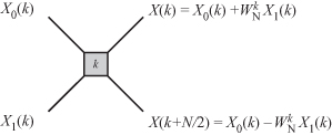
Figure 19.4 Evaluation of a decimation-in-time eight-point DFT based on two four-point DFTs.

We indicated in the previous section that when N is an integer power of two, then the FFT can be evaluated by successively splitting the input data sequence in even and odd parts. Table 19.1 shows the successive splitting of a 16-point input data sequence. Each splitting divides the input into even and odd parts. The first column of the table shows the binary address or order of the input data samples. The second column shows the data assuming it arrives, or stored, in the natural order in sequence. The third column is the data after the first splitting into even and odd data of length N/2 = 4. The fourth column shows the data after the second splitting. Note that at this stage, each sequence contains only two data samples where we can simply do a two-point DFT using additions and subtractions since and . The fifth column shows the binary representation of the data index. This could be considered as their memory location, for example.

Table 19.1 Successive Splitting of Input Data in Even and Odd Parts

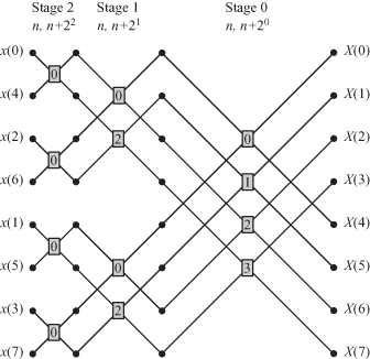
Compare the first and the last columns of the table. It shows what is known as bit reversal. The two-point DFTs need input data that is the bit reverse of the natural order; therefore, location 1, which is 001 in binary, will be bit reversed to 100, which corresponds to input sample x(4). The eight-point FFT will use the information in Table 19.1 for its operation. We start with the two-point DFTs, whose input data correspond to the data in the fourth column (second splitting). The outputs will be fed to four-point DFTs, whose input data correspond to the data in the third column (first splitting). The reader can try constructing a similar table for a 16-point DFT.

Now we are ready to construct the DG for the eight-point decimation-in-time FFT algorithm, which is shown in Fig. 19.5. The eight-point FFT consists of three stages since log₂ 8 = 3. Each stage contains N/2 = 4 butterfly operations. Stage 2 performs two-point DFT processes and the butterflies at that stage operate on data whose indices are 2² apart. Stage 1 performs two-point DFT processes and the butterflies at that stage operate on data whose indices are 2¹ apart. Stage 0 performs two-point DFT processes and the butterflies at that stage operate on data whose indices are 2⁰ apart. The sequence of operations is from left to right; therefore, all operations in stage 2 must be completed before operations in stage 1 can start.

Figure 19.5 DG for an eight-point decimation-in-time FFT algorithm.

The FFT algorithm we described here applied to the case when N is an integer power of two, that is, N = 2^r. This is called radix-2 FFT algorithm because the input samples are divided into two parts and the butterfly operations involve two inputs and produce two outputs. Higher radix FFTs are possible. For example, radix-4 FFT assumes N = 4^r and divides the input data into four parts and the butterflies operate on four input samples and produce four output samples. The outputs of the butterfly would be related to the inputs according to the expressions

(19.14)

(19.15)

(19.16)

(19.17)