
11.7 DESIGN SPACE EXPLORATION: CHOICE OF BROADCASTING VERSUS PIPELINING VARIABLES
At this point, we know we have three variables, M1, M2, and M3, for our matrix multiplication algorithm. We have a choice whether to broadcast or to pipeline each variable. Thus, we have eight different possible design choices for the implementation of our algorithm. Some of these choices might not be feasible though. In what follows, we show only one of those choices, but the reader can explore the other choices following the same techniques we provide here.
Broadcasting an output variable means performing all the calculations necessary to produce it at the same time. It is not recommended to broadcast output variables since this would result in a slower system that requires gathering all the partial outputs and somehow using them to produce the output value. To summarize, if v is an input variable, all points in B potentially use the same value of v. If v is an output variable, all points in B are potentially used to produce v.
Broadcasting an input variable means making a copy available to all processors at the same time. This usually results in the algorithm completing sooner. It is always preferable to broadcast input variables since this only costs using buses to distribute the variables. Data broadcast could be accomplished in hardware using a system-wide bus or an interconnection network capable of broadcasting a single data item to all the processing elements (PEs). In software, data broadcast could be accomplished using a broadcast message to all threads or using a shared memory.
11.7.1 Feeding/Extraction Point of a Broadcast Variable
The problem we address in this section is as follows. Assume we are given a particular instance M2(c1, c2) of the input variable M2. We want to determine a point in ![]() to feed this input instance. We choose this point at the boundaries of
to feed this input instance. We choose this point at the boundaries of ![]() . To find such a point, we find the intersection of the broadcast subdomain of M2 with
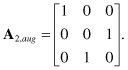
. To find such a point, we find the intersection of the broadcast subdomain of M2 with ![]() . The intersection point is found by augmenting the dependence matrix A2 to make it full rank. We use one of the three candidate facets from the lower or upper hull. We choose to feed the variable from the lower hull facets described by Eqs. 11.13, 11.14, or 11.15. Only the facet described by Eq. 11.14 increases the rank of A2 as it is linearly independent for all its rows. Now our augmented matrix will be
. The intersection point is found by augmenting the dependence matrix A2 to make it full rank. We use one of the three candidate facets from the lower or upper hull. We choose to feed the variable from the lower hull facets described by Eqs. 11.13, 11.14, or 11.15. Only the facet described by Eq. 11.14 increases the rank of A2 as it is linearly independent for all its rows. Now our augmented matrix will be
(11.40)
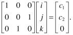
The intersection point is specified by the equation
(11.41)
![]()
where c is the intersection point in the domain ![]() . Specifically, we can write
. Specifically, we can write
(11.42)
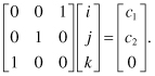
Solving the above three simultaneous equations in the three unknowns i, j, and k, we get the intersection point for variable M2(c1, c2) as
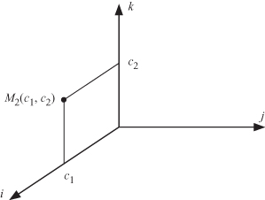
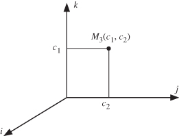
Thus, instance M2(c1, c2) is fed to the system at the point with coordinates given by the above equation. Figure 11.3 shows the feeding point for supplying variable instance M2(c1, c2) to the 3-D computation domain ![]() for the matrix multiplication algorithm.
for the matrix multiplication algorithm.
Figure 11.3 The feeding point for supplying variable instance M2(c1, c2) to the 3-D computation domain ![]() for the matrix multiplication algorithm.
for the matrix multiplication algorithm.
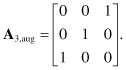
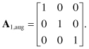
Let us now find the feeding point for input variable instance M3(c1, c2). We also choose to augment the dependence matrix A3 from one of the facets of the lower hull. Only the facet described by Eq. 11.13 increases the rank of M3 as it is linearly independent for all its rows. We should not spend too much time worrying about whether to choose the augmenting facet from the lower or upper hulls since broadcasting does not really care where the bus is fed from as long as all processors receive the data. Now our augmented matrix will be
(11.44)
The intersection point is specified by the equation
(11.45)
![]()
where c is the intersection point in the domain ![]() . Specifically, we can write
. Specifically, we can write
(11.46)
Solving the above three simultaneous equations in the three unknowns we get the intersection point for variable M3(c1, c2) as
Thus, instance M3(c1, c2) is fed to the system at the point with coordinates given by the above equation. Figure 11.4 shows the feeding point for supplying variable instance M3(c1, c2) to the 3-D computation domain ![]() for the matrix multiplication algorithm.
for the matrix multiplication algorithm.
Figure 11.4 The feeding point for supplying variable instance M3(c1, c2) to the 3-D computation domain ![]() for the matrix multiplication algorithm.
for the matrix multiplication algorithm.
11.7.2 Pipelining of a Variable
We can introduce pipelining to the broadcast subdomain B of variable v by dedicating some of the basis vectors of B as data pipeline directions. The remaining basis vectors will remain broadcast directions. When we assign some basis vectors to describe our pipelining, the remaining basis vectors define a reduced broadcast subdomain over which variable v is still broadcast. In this way, we can mix pipelining and broadcasting strategies to propagate (or evaluate) the same input (or output) variable.
For our matrix multiplication algorithm, we choose to pipeline our output data samples M1(c1, c2). Now pipelined data travels from one point in ![]() to another along a given direction. We need to determine the directions of data pipelining, which are the nullspace of the dependence matrix for M1, that is, along the direction given by the vector given by e = [0 0 1]t. We need to determine two distinct intersection points of B with
to another along a given direction. We need to determine the directions of data pipelining, which are the nullspace of the dependence matrix for M1, that is, along the direction given by the vector given by e = [0 0 1]t. We need to determine two distinct intersection points of B with ![]() . One point is used to initialize the pipeline. The other point is used to extract the pipeline output. To find the intersection points, we augment the dependence matrix A1 using lower and upper hull facets. The only possible candidates for augmenting A1 are given by Eqs. 11.9 and 11.15.
. One point is used to initialize the pipeline. The other point is used to extract the pipeline output. To find the intersection points, we augment the dependence matrix A1 using lower and upper hull facets. The only possible candidates for augmenting A1 are given by Eqs. 11.9 and 11.15.
Now our augmented matrix will be
(11.48)
We can write the two augmented matrices using the expression
(11.49)
![]()
We can explicitly write the above two equations as
(11.50)
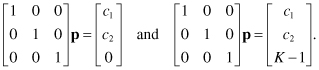
The solution for the above two equations gives
Thus, we know the possible locations of initializing or extracting the pipeline data in the computation domain. The detailed method to obtain the extraction points and the feeding points at the projected domain will be discussed later in this chapter.