![14.12 INTERPOLATOR DAG FOR s1 = [1 0]](https://imgdetail.ebookreading.net/cover/cover/software_development/EB9780470934630.jpg)
14.12 INTERPOLATOR DAG FOR s1 = [1 0]
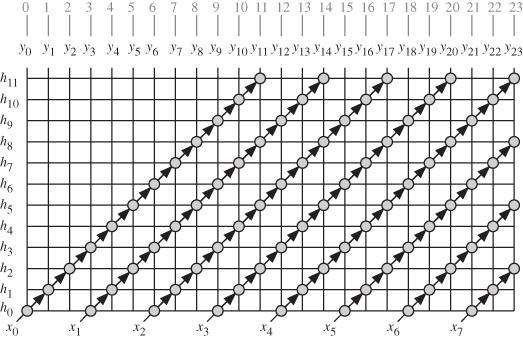
The DAG corresponding to s1 is shown in Fig. 14.13. The equitemporal planes are indicated by the gray lines and the time index values are indicated by the grayed numbers associated with the equitemporal planes. We note from the figure that a maximum of four tasks or nodes is active at any time step. It should also be noted that the time values are associated with the high data rate of the interpolator output. We have three possible valid projection vectors:
(14.36)
![]()
(14.37)
![]()
(14.38)
![]()
Figure 14.13 1-to-L interpolator DAG for the case when L = 3, N = 12, and s1 = [1 0].
These projection directions correspond to the projection matrices
(14.39)
![]()
(14.40)
![]()
(14.41)
![]()
We consider only the design corresponding to d1a since the other two designs will be more complex and will not lead to a better task workload. A point in the DAG given by the coordinate p = [n k]t will be mapped into the point in the reduced or projected ![]() given by
given by
(14.42)
![]()
Output sample calculations are all performed at the same time step. In that sense, the input samples are pipelined and output samples are broadcast. We note however, that each task is active once every L time steps. In order to reduce the number of nodes, we modify the linear projection operation above to employ a nonlinear projection operation:
(14.43)
![]()
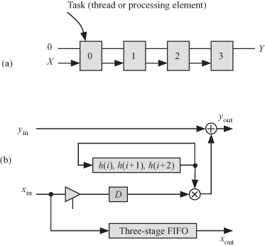
Figure 14.14 shows the implementation of Design 1a. Figure 14.14a shows the ![]() , where input samples are pipelined between the tasks and the partial results for the output samples are broadcast among the tasks. Note that the number of tasks required is N/L. Figure 14.14b shows the task detail. Each task is simple in hardware and in control structure. Each task accepts an input sample every L time steps and forwards the input to the next task after a delay of L time steps. All tasks pipeline the incoming data x(n) at the low data rate and perform the filtering operation at the high data rate. The output is obtained from the rightmost task at each time step.
, where input samples are pipelined between the tasks and the partial results for the output samples are broadcast among the tasks. Note that the number of tasks required is N/L. Figure 14.14b shows the task detail. Each task is simple in hardware and in control structure. Each task accepts an input sample every L time steps and forwards the input to the next task after a delay of L time steps. All tasks pipeline the incoming data x(n) at the low data rate and perform the filtering operation at the high data rate. The output is obtained from the rightmost task at each time step.
Figure 14.14 Interpolator Design 1a for s1, d1a, N = 12, and L = 3. (a) Resulting ![]() . (b) Task processing detail. In the figure FIFO is first-in-first-out buffer.
. (b) Task processing detail. In the figure FIFO is first-in-first-out buffer.