
Chapter 20. Textures and Texture Mapping
20.1. Introduction
As we said in Chapter 1, texture mapping can be used to add detail to the appearance of an object. Texture mapping has little to do with either texture (in the sense of the roughness or smoothness you feel when you touch something) or maps; the term is an artifact of the early history of graphics.
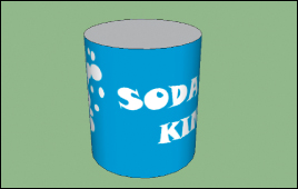
A typical use of texture mapping is to make something that looks painted, like a soft-drink can. First you make a 2D image I that looks like an unrolled version of the vertical sides of the can (see Figure 20.1). Then you give the image coordinates u and v that range from 0 to 1 in the horizontal and vertical directions. Then you model a cylinder, perhaps as a mesh of a few hundred polygons based on vertex locations like

where r is the can’s radius, h is its height, and i = 0, ..., 10 and j = 0, ..., 5 (see Figure 20.2). A typical triangle might have vertices P11, P12, and P21.
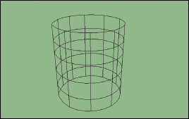
Now you also assign to each vertex so-called uv-coordinates: a u- and a v-value at each vertex. In this example, the u-coordinate of vertex Pij would be i/10 and the v-coordinate would be j/5. Notice that the vertices P0,0 and P10,0 are in identical locations (at the “seam” of the can), but they have different uv-“coordinates.” Because coordinates should be unique to a point (at least in mathematics), it might make more sense to call these uv-“values,” but the term “coordinates” is well established. We will, however, refer henceforth to texture coordinates rather than “uv-coordinates,” both because sometimes we use one or three rather than two coordinates, and because the tying of concepts to particular letters of the alphabet can be problematic, as in the case where a single mesh has two different sets of texture coordinates assigned to it.
When it comes time to render a triangle, it gets rasterized, that is, broken into tiny fragments, each of which will contribute to one pixel of the final result. The coordinates of these fragments are determined by interpolating the vertex coordinates, but at the same time, the renderer (or graphics card) interpolates the texture coordinates. Each fragment of a triangle gets different texture coordinates. During the rendering step in which a color is computed for the fragment, often based on the incoming light, the direction to the eye, the surface normal, etc., as in the Phong model of Chapter 6, the material color is one of the items needed in the computation. Texture mapping is the process of using the texture coordinate for the fragment to look up the material color in the image I rather than just using a fixed color. Figure 20.3 shows the effect.
We’ve omitted many details from this brief description, including a step in which fragments are further reduced to samples, but it conveys the essential idea, which has been generalized in a great many ways.
A value (e.g, the color) associated to a fragment of a triangle is almost always the result of a computation, one that has many parameters such as the incoming light, the surface normal, the vector from the surface to the eye, the surface color (or other descriptions of surface scattering like the bidirectional reflectance distribution function or BRDF), etc. Ordinarily, many of these parameters either are constants or are computed by interpolating values from the triangle’s vertices. If instead we barycentrically interpolate some texture coordinates from the triangle vertices, these coordinates can be used as arguments to one or more functions whose values are then used as the parameters. A typical function is “look up a value at location (u, v) in an image whose domain is parameterized by 0 ≤ u, v ≤ 1,” but there are many other possibilities.
Much of this chapter elaborates on this idea, discussing the parameters that can be varied, the codomains for texture coordinates (i.e., the meaning of the values that they take on), and mechanisms for defining mappings from a mesh to the space of coordinates.
You’ll notice that this entire notion of “texture mapping” is really just a name for indirection as applied in a specific context: We use an index (the texture coordinates) to determine a value. This determination may be performed by a table lookup (as in the case of the soft-drink can above, where the texture image serves as the “table”) or by a more complex computation, in which case it’s often called procedural texturing.
An example of the power of various mapping operations is given by this book’s cover image, in which almost every object you see has had multiple maps applied to it—color, texture, displacement, etc.—resulting in a visual richness that would be almost impossible to achieve otherwise.
20.2. Variations of Texturing
We’ll illustrate several variations on the idea of texture mapping, working with the Phong reflection model as an exemplar. The ideas we present are largely independent of the reflection model, and they apply more generally. Because the unit square 0 ≤ u, v ≤ 1 occurs so often in this chapter, we’ll give it a name, U, which we’ll use in this chapter only.
Recall that in the Phong model of Chapter 6, the light scattered from a surface is defined by various constants (the diffuse reflection coefficient kd, the specular reflection coefficient ks, the diffuse and specular colors Cd and Cs, and the specular exponent n), dot products of various unit vectors, including the direction vector to the light source, the direction vector from the surface to the eye, the surface normal vector, and finally, the arriving light. There is also, in some versions of the model, an ambient term, modeled by ka and Ca, indicating an amount of light emitted by the surface independent of the arriving light. Each of these things—the constants, the vectors, and even the way you compute the dot product—is a candidate for mapping.
20.2.1. Environment Mapping
If our surface is mirrorlike (i.e., kd = ka = 0, and n is very large, or even infinite), then the light scattered toward the eye, as determined by the Phong model, is computed by reflecting the eye ray through the surface normal to get a ray that may point toward a light source (in which case light is scattered) or not. If all sources are point sources, this tends to result in no rendered reflection at all, since the probability of a ray hitting any particular source is zero. If the sources are area sources, we see them reflected in our object.
We can replace our model of light arriving at the surface point P from one based on a few point or area sources to one based on a texture lookup: We can treat the reflected eye vector as a point of the unit sphere, and use it to index into a texture-mapped sphere to look up the arriving light. In practical terms, if we write this eye vector in polar (world) coordinates, (θ, φ), for instance, we can use ![]() to index into an environment map that contains, at location (u, v), the light arriving from the corresponding direction.
to index into an environment map that contains, at location (u, v), the light arriving from the corresponding direction.
Notice that as the point P moves, the light arriving at the point P from direction v doesn’t change. Thus, this environment map is useful for modeling the specular reflection of an object’s surroundings, but it is not good for modeling reflections of nearby objects, where the direction from P to some object will change substantially as we vary P.
Where do we get an environment map in the first place? A fisheye-lens photograph taken from the center of a scene can provide the necessary input, although the mapping from pixels in the photograph to pixels in the environment map requires careful resampling. In practice, it’s common to use multiple ordinary photographs, and a rather different mapping strategy from the one we’ve suggested here, but the key idea—doing a lighting “lookup” rather than iterating over a small list of point or area lights—remains the same.
Debevec has written an interesting first-person history of reflection mapping in general [Deb06], tracing its first use in graphics to a paper by Blinn and Newell in 1976 [BN76], which is long before digital photographs were available! The “environment map” in this case was a scene created in a drawing program.
We’ve carefully suggested using environment mapping in a ray tracer for describing the lighting of a mirrorlike surface. What would be entailed in using environment mapping on a glossy surface? A diffuse one? Would it substantially increase the computation time over that of a simpler model in which the light was specified by a few point and area lights?
20.2.2. Bump Mapping
In bump mapping, we fiddle with another of the ingredients in the Phong model: the surface normal, n. A typical version of this uses texture coordinates on a model to look up a value in a bump map image and uses the resultant values to alter the normal vector a little.
The exact meaning assigned to the RGB values from this image depends on the implementation, but a simple version uses just R and G to “tilt” the normal vector as follows. We’ll assume that at each surface point P we have a pair of unit vectors t1 and t2 that are tangent to the surface, are mutually perpendicular, and vary continuously across the surface. In theory, it may be impossible to find such a pair of vector fields (see Chapter 25), and in Section 20.3 we’ll discuss this further, but in practice usually only the continuity assumption is violated, and only at a few isolated points. For example, on the unit sphere, tangents to the lines of constant latitude and constant longitude can play the role of t1 and t2, failing the continuity requirement only at the north and south poles. If we arrange to not perturb the normal vector at either pole, then the lack of continuity of t1 and t2 has no effect.
With t1 and t2 in hand, we’ll show how to adjust the normal vector. The R and G values from the bump map, typically bytes representing values –128, ..., 127, or unsigned bytes representing 0 to 255, are adjusted to range from –1 to 1 by writing (in the first case)
and a corresponding expression for g. (The loss of –128 as a distinct value is deliberate. If we’d divided by 128, we could not represent +1.0.)
We can now adjust the normal vector n, as shown in Figure 20.4, by computing
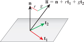
Figure 20.4: The vector ![]() will be normalized to produce the new normal n′; the values r and g (for “red” and “green”) vary across the surface, and are looked up in a texture map.
will be normalized to produce the new normal n′; the values r and g (for “red” and “green”) vary across the surface, and are looked up in a texture map.
At the extreme (when r = g = 1) this tilts the normal vector by about 54°. If a larger amount of tilt is needed, one can redefine r and g to range from –2 to 2, or even more.
One advantage to this scheme, originally proposed by Blinn [BN76], is that n + rt1 + gt2 can never be zero, because its dot product with n is one. This means that it can always be normalized.
By the way, the particular form we’ve described for converting image-pixel values into values between –1.0 and 1.0 is part of the OpenGL standard and is called the signed normalized fixed-point 8-bit representation (see Chapter 14). There are other standard representations as well, using more bits per pixel, unsigned rather than signed values, etc. There’s nothing sacred about any of these. They’ve proven to be convenient over the years, so they become standardized.
A more direct approach is to store in the texture image three floating-point numbers (i.e., we treat the bits in the red channel as a float, and do the same for green and blue), and use this triple of numbers as the coordinates of the (unnormalized) normal vector, from which we can compute n; this is one of the most common approaches today.
![]() It’s possible to specify a set of normal vectors that are not actually consistent with each other, that is, they do not form the normal vector field for any surface (see Exercise 20.2). When rendered, these can look peculiar. So a third approach to bump mapping is to have the texture contain a height for each texture coordinate (u, v), indicating that we are to imagine that the surface is displaced from its current position by that amount along the original normal vector. The resultant surface (which is never actually created!) has tangent vectors in the u- and v-directions (i.e., the direction of greatest increase of u, and correspondingly of v), whose cross product we compute and use as the “normal” vector during shading computations. This clearly requires substantially more computation, but far less bandwidth, since we need only one value per location rather than two or three.
It’s possible to specify a set of normal vectors that are not actually consistent with each other, that is, they do not form the normal vector field for any surface (see Exercise 20.2). When rendered, these can look peculiar. So a third approach to bump mapping is to have the texture contain a height for each texture coordinate (u, v), indicating that we are to imagine that the surface is displaced from its current position by that amount along the original normal vector. The resultant surface (which is never actually created!) has tangent vectors in the u- and v-directions (i.e., the direction of greatest increase of u, and correspondingly of v), whose cross product we compute and use as the “normal” vector during shading computations. This clearly requires substantially more computation, but far less bandwidth, since we need only one value per location rather than two or three.
20.2.3. Contour Drawing
This example differs from the previous ones, because each surface point will have only one texture coordinate. A point P of a smooth surface is on a contour if the ray from P to the eye E, r = E – P, is perpendicular to the surface normal n. Thus, to render a surface by drawing its contours, all we must do is compute this dot product, and when it’s near zero, make a black mark on the image, or leave the image white otherwise. To do so we make a one-dimensional texture map like the one shown in Figure 20.5. And as a texture coordinate, we compute
As the dot product ranges from –1 to 0 to 1, u ranges from 0 to ![]() to 1. At u =
to 1. At u = ![]() , the dark color we find in the texture map creates a dark spot in the image. To be clear: This “rendering” algorithm involves no lighting or reflection or anything like that. It’s simply following the rule that we can draw the contours of an object to make a reasonably effective picture of it. An actual implementation of a slightly fancier version of this algorithm is given in Section 33.8.
, the dark color we find in the texture map creates a dark spot in the image. To be clear: This “rendering” algorithm involves no lighting or reflection or anything like that. It’s simply following the rule that we can draw the contours of an object to make a reasonably effective picture of it. An actual implementation of a slightly fancier version of this algorithm is given in Section 33.8.
20.3. Building Tangent Vectors from a Parameterization
We’ll now describe how to find a frame (i.e., a basis) for the tangent space at each point of a parameterized smooth surface, and then, working by analogy, describe a similar construction for a mesh.
The sphere, which we’ll use as our smooth example, is often parameterized by
where θ ranges from 0 to 2π, and φ ranges from –![]() to
to ![]() .
.
If we hold θ constant in P(θ, φ) and vary φ, we get a line of longitude; similarly, if we hold φ constant and vary θ, we get a line of latitude. If we compute the tangent vectors to these two curves, we get
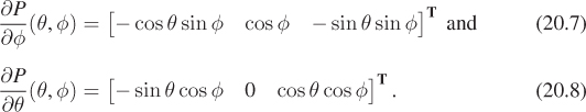
These vectors, drawn at the location P(θ, φ), are tangent to the sphere at that point, and they happen to be perpendicular as well (see Figure 20.6). Except at the north and south poles (where cos(φ) = 0), the vectors are nonzero, so the two of them constitute a frame at almost every point. In general, it’s topologically impossible to find a smoothly varying frame at every point of an arbitrary surface, so our situation, with a frame at almost every point, is the best we can hope for.
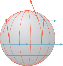
Figure 20.6: The sphere, with vertical lines of constant θ and horizontal lines of constant φ drawn in red and blue, respectively, and tangent vectors to those curves at a few points.
In general, if we have any surface parameterized by a function like P of two variables—say, u and v—then ![]() and
and ![]() are a pair of vectors at the point (u, v) that form a basis for the tangent plane there, except in two circumstances: One of the vectors may be zero, or the two vectors may be parallel. In both situations, the parameterization is degenerate in some way, and for “nice” surface parameterizations this should happen only at isolated points. To get an even nicer framing, you can normalize the first vector and compute its cross product with the normal vector to get the second; the result will be an orthonormal frame at every place where the first vector is nonzero.
are a pair of vectors at the point (u, v) that form a basis for the tangent plane there, except in two circumstances: One of the vectors may be zero, or the two vectors may be parallel. In both situations, the parameterization is degenerate in some way, and for “nice” surface parameterizations this should happen only at isolated points. To get an even nicer framing, you can normalize the first vector and compute its cross product with the normal vector to get the second; the result will be an orthonormal frame at every place where the first vector is nonzero.
We can now proceed analogously on a mesh for which each vertex has xyz-coordinates and uv-texture coordinates assigned. We’ll do so one face at a time. The assignment of (u, v) coordinates to each vertex defines an affine (linear-plus-translation) map from the xyz-plane of the triangular face to the uv-plane (or vice versa). We’d like to know what the curve of constant u or constant v looks like, in analogy with the curves of constant θ and φ in the sphere example above, so that we can compute the tangent vectors to these curves. Fortunately, for an affine map a curve of constant v is just a line; all we need to do is find the direction of this line.
Suppose the face has vertices P0, P1, and P2, with associated texture coordinates (u0, v0), (u1, v1), and (u2, v2). We’ll study everything relative to P0, so we define the edge vectors w1 = P1 – P0 and w2 = P2 – P0, and similarly define Δui = ui – u0 (i = 1, 2), and similarly for v (see Figure 20.7).
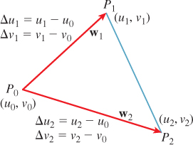
Since v varies linearly (or affinely, to be precise) along each edge vector, consider the vector w = Δv2w1–Δv1w2. How much does v change along this vector? It changes by Δv1 along w1, so along the first term, it changes by Δv2Δv1; a similar argument shows that on the second term, it changes by Δv1Δv2. Hence on the sum, w, v remains constant. We’ve found a vector on which v is constant! We can do the same thing for u, so the frame for this triangle has, as its two vectors,
Unfortunately, if we perform the same computation for an adjacent triangle, we’ll get a different pair of vectors. We can, however, at each vertex of the mesh, average the f1 vectors from all adjacent faces and normalize, and similarly for the f2 vectors. We can then interpolate these averaged values over the interior of each triangle. There’s always the possibility that either one of the average vectors at a vertex will be zero, or that when we interpolate we’ll get a zero at some interior point of a triangle. (Indeed, this will have to happen for most closed surfaces except those that have the topology of a torus.) But this is just the piecewise-linear version of the problems we already encountered for smooth maps. If we’re using this framing to perform bump mapping, we’ll want to avoid assigning a nonzero coefficient at any point at which one of the frame vectors is zero.
20.4. Codomains for Texture Maps
The texture values that we define at vertices, and which are interpolated across faces of a triangular mesh, are represented as numbers. When we have two texture coordinates u and v, we’re implicitly defining a mapping from our mesh to a unit square in the uv-plane. The codomain of the texture-coordinate assignment in this case is the unit square. There are two generalizations of this.
First, some systems allow texture coordinates to take on values outside the range U = {(u, v)|0 ≤ u ≤ 1, 0 ≤ v ≤ 1}. Before the coordinates are actually used, they are reduced mod 1, that is, u is converted to u – floor(u), and similarly for v. The net effect can be viewed in one of two ways.
1. The uv-plane, rather than having a single image placed in the unit square, is tiled with the image. Our texture coordinates define a map into this tiled plane (see Figure 20.8).
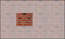
Figure 20.8: The texture image, shown dark, can be replicated across the whole plane (shaded squares) so that texture coordinates outside the unit square can be used.
2. The edges of the unit square defined by the lines u = 1 and u = 0 are treated as identical; the square is effectively rolled up into a cylinder. Similarly, the lines v = 1 and v = 0 are identified with each other, rolling up the cylinder into a torus (see Figure 20.9). If you like, you can consider the point (u, v) as corresponding to the point that’s 2πu of the way around the torus in one direction, and 2πv around it in the other direction, with the texture stretched over the whole torus. The texture coordinates define a mapping from your object to the surface of a torus.

Figure 20.9: The sides of the square are identified to form a cylinder; the ends of the cylinder are then identified to make a torus.
For either interpretation to make sense, the texture-map values on the right-hand side of the unit square must match up nicely with those on the left (and similarly for the top and bottom), or else the texture will be discontinuous on the u = 0 circle of the torus, and similarly for the v = 0 circle. Furthermore, any filtering or image processing you do to the texture image must involve a “wraparound” to blend values from the left with those from the right, and from top to bottom as well.
The second generalization was already suggested by the second version of bump mapping: The texture coordinates define a map of your object onto a surface in some higher-dimensional space. In the case of bump mapping, each object point is sent to a unit vector, that is, the codomain is the unit sphere within 3-space.
In general, the appropriate target for texture coordinates depends on their intended use.
Here are a few more examples.
• You can use the actual coordinates of each point as texture coordinates (perhaps scaling them to fit within a unit cube first). If you then generate a cubical “image” that looks like marble or wood, and use the texture value as the color at each point, you can make your object look as if it were carved from marble or wood. In this case, your texture uses a lot of memory, but only a small part of it is ever used to color the model. The codomain is a cube in 3-space, but the image of the texture-coordinate map is just the surface of your object, scaled to fit within this cube.
• A nonzero triple (u, v, w) of texture coordinates (typically a unit vector) is converted to (u/t, v/t, w/t) where t = 2 max(|u|, |v|, |w|); the result is a triple with one coordinate equal to ±![]() , and the other two in the range
, and the other two in the range ![]() , that is, a point on the face of the unit cube. Each one of the six faces of the cube (corresponding to u, v, or w being +
, that is, a point on the face of the unit cube. Each one of the six faces of the cube (corresponding to u, v, or w being +![]() or –
or –![]() is associated to its own texture map. This provides a texture on the unit sphere in which the distortion between each texture-map “patch” and the sphere is relatively small. This structure is called a cube map, and it is a standard part of many graphics packages; it’s the currently preferred way to specify spherical textures. Alternatives, like the latitude-longitude parameterization of the sphere, are useful in situations where the high distortion near the poles is unimportant (as in the case of a world map, where the area near the poles is all white).
is associated to its own texture map. This provides a texture on the unit sphere in which the distortion between each texture-map “patch” and the sphere is relatively small. This structure is called a cube map, and it is a standard part of many graphics packages; it’s the currently preferred way to specify spherical textures. Alternatives, like the latitude-longitude parameterization of the sphere, are useful in situations where the high distortion near the poles is unimportant (as in the case of a world map, where the area near the poles is all white).
• In the event that the cube map needs to be regenerated often (e.g., if it’s an environment map generated by rendering a changing scene from the point of view of the object), rendering the scene in six different views may be more work than you want to do. A natural alternative is to make two hemispherical renderings, recording light arriving from direction [x y z]T at position ![]() in one image for y ≥ 0 and another for y ≥ 0. Each of these renderings uses only π/4 ≈ 79% of the area of the unit square, but they’re very easy to compute and use. (An alternative two-patch solution is the dual paraboloid of Exercise 20.4.)
in one image for y ≥ 0 and another for y ≥ 0. Each of these renderings uses only π/4 ≈ 79% of the area of the unit square, but they’re very easy to compute and use. (An alternative two-patch solution is the dual paraboloid of Exercise 20.4.)
20.5. Assigning Texture Coordinates
How do we specify the mapping from an object to texture space? The great majority of standard methods start by assigning texture coordinates at mesh vertices and using linear interpolation to extend over the interior of each mesh face. We often (but not always) want that mapping to have the following properties.
• Piecewise linear: As we said, this makes it possible to use interpolation hardware to determine values at points other than mesh vertices.
• Invertible: If the mapping is invertible, we can go “backward” from texture space to the surface, which can be helpful during operations like filtering.
• Easy to compute: Every point at which we compute lighting (or whatever other computation uses mapping) will have to have the texture-coordinate computation applied to it. The more efficient it is, the better.
• Area preserving: This means that the space in the texture map is used efficiently. Even better, when we need to filter textures, etc., is to have the map be area-and-angle preserving, that is, an isometry, but this is seldom possible. A compromise is a conformal mapping, which is angle preserving, so that at each point, it locally looks like a uniform scaling operation [HAT+00].
The following are examples of some common mappings.
• Linear/planar/hyperplanar projection: In other words, you just use some or all of the surface point’s world coordinates to define a point in texture space. Peachey [Pea85] called these projection textures. The wooden ball in Figure 20.10 was made this way: The texture shown at the right on the yz-aligned plane was used to texture the ball by coloring the ball point (x, y, z) with the image color at location (0, y, z).
• Cylindrical: For objects that have some central axis, we can surround the object with a large cylinder and project from the axis through the object to the cylinder; if the point (x, y) projects to a point (r, θ, z) in cylindrical coordinates (r being a constant), we assign it texture coordinates (θ, z). More precisely, we use coordinates ![]() ,
, ![]() , where the clamp(x, a, b) returns x if a ≤ x ≤ b, a if x < a, and b if x > b.
, where the clamp(x, a, b) returns x if a ≤ x ≤ b, a if x < a, and b if x > b.
• Spherical: We can often pick a central point within an object and project to a sphere in much the same way we did for cylindrical mapping, and then use suitably scaled polar coordinates on the sphere to act as texture coordinates.
• Piecewise-linear or piecewise-bilinear on a plane from explicit per-vertex texture coordinates (UV): This is the method we’ve said was most common, but it requires, as a starting point, an assignment of texture coordinates to each vertex. There are at least four ways to do this.
– Have an artist explicitly assign coordinates to some or all vertices. If the artist only assigns coordinates to some vertices, you need to algorithmically determine interpolated coordinates at other vertices.
– Use an algorithmic approach to “unfold” your mesh onto a plane in a distortion-minimizing way, typically involving cutting along some (algorithmically determined) seams. This process is called texture parameterization in the literature. Some aspects of texture parameterization may also be used in the interpolation of coordinates in the artist-assigned texture-coordinate methods above.
– Use an algorithmic approach to break your surface into patches, each of which has little enough curvature that it can be mapped to the plane with low distortion, and then define multiple texture maps, one per patch. The cube-map approach to texturing a sphere is an example of this approach. Filtering such texture structures requires either looking past the edge of a patch into the adjacent patch, or using overlapping patches, as mathematicians do when they define manifold structures. The former approach uses textures efficiently, but involves algorithmic complications; the latter wastes some texture space, but simplifies filtering operations.
– Have an artist “paint” the texture directly onto the object, and develop a coordinate mapping (or several patches as above) as the artist does so. This approach is taken by Igarashi et al. in the Chameleon system [IC01]. In a closely related approach, the painted texture is stored in a three-dimensional data structure so that the point’s world-space coordinates serve as the texture coordinates. These are used to index into the spatial data structure and find the texture value that’s stored there. Detailed textures are stored by using a hierarchical spatial data structure like an octree: When the artist adds detail at a scale smaller than the current octree cell, the cell is subdivided to better capture the texture [DGPR02, BD02].
• Normal-vector projection onto a sphere: The texture coordinates assigned to a point (x, y, z) with unit normal vector n = [nx ny nz]T are treated as a function of nx, ny, and nz, either as the angular spherical polar coordinates of the point (nx, ny, nz) (the radial coordinate is always 1), or by using a cube-map texture indexed by n.
There are even generalizations in which the texture coordinates are not assigned to a point of an object, but instead are a function of the point and some other data. Environment mapping is one of these: In this case the texture coordinates are derived from the reflected eye vector on a mirrorlike surface.
There are also generalizations in which the Noncommutativity principle is applied: Certain operations, like filtering multiple samples to estimate average radiance arriving at a sensor pixel, can be exchanged with other operations, like the reflection computation used in environment mapping, without introducing too much error. If you want to environment-map a nonmirror surface, you’ll want to compute many scattered rays from the eye ray, look up arriving radiance for each of them in the environment map, multiply appropriately by a BRDF value and cosine, and average. You can instead start with a different environment map that at each location stores the average of many nearby samples from the original environment map (i.e., a blurred version of the original). You can then push one sample of this new map through the BRDF and cosine to get a radiance value: You’ve swapped the averaging of samples with the convolution of light against the BRDF and cosine. These operations do not, in fact, commute, so the answers you produce will generally be incorrect. But they are often, especially for almost-diffuse surfaces, quite good enough for most purposes, and they speed up the rendering substantially. Approaches like this are grouped under the general term reflection mapping.
As an extreme example, for a diffuse surface the only characteristic of the arriving light that matters is irradiance—the cosine-weighted average radiance over the visible hemisphere [RH01]. From an environment map, one can compute the average for every possible direction, and use this irradiance map to rapidly compute light reflected from a diffuse surface, assuming that the light arrives from far enough away that the irradiance is a function of direction only. Figure 20.11 shows such an irradiance map, and Figure 20.12 shows a figure illuminated by it.
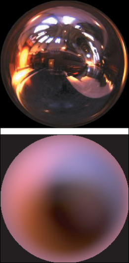
Figure 20.11: Top: A sphere map of light arriving at one point in Grace Cathedral (Photograph used with permission. Copyright 2012 University of Southern California, Institute for Creative Technologies.) Bottom: An irradiance map formed from that sphere map (Courtesy of Ravi Ramamoorthi and Pat Hanrahan, © 2001 ACM, Inc. Reprinted by permission.)
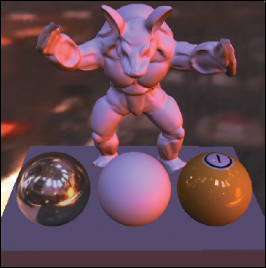
Figure 20.12: Several objects illuminated by the irradiance map, represented in a compact approximation (Courtesy of Ravi Ramamoorthi and Pat Hanrahan, © 2001 ACM, Inc. Reprinted by permission.)
Describe the appearance of a pure-white, totally diffuse sphere, illuminated by the irradiance map of Figure 20.11, top, rendered with a parallel projection in the same direction as the view shown for the irradiance map.
20.6. Application Examples
Now that we’ve described the general idea of texture mapping (assigning texture coordinates to object points, followed by evaluating functions on these coordinates, often by interpolation of image values), let’s look at a range of applications. Table 20.1 presents these, listing for each application the property that is being mapped, the map being used, and the name of the resultant technique. We use the name “UV” to indicate some kind of surface parameterization.
20.7. Sampling, Aliasing, Filtering, and Reconstruction
When we render a scene in which there is texture mapping, no matter how simple or complex the mapping scheme is, problems with sampling and aliasing can arise.
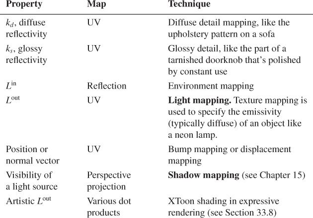
Figure 20.13 shows a very simple example, a ray-traced scene in which there’s no lighting, but there is a single infinite ground plane and an infinite sky plane. The sky is blue; the ground has a checkerboard pattern. The color for a ray traced into the scene is therefore either blue, black, or white.
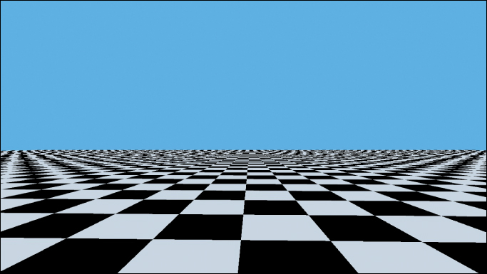
Figure 20.13: Aliasing arising from single-sample ray tracing of a checkerboard texture (Courtesy of Kefei Lei).
Even though the checkerboard texture is absolutely perfect, in the sense that it’s represented by a function, namely, “Is floor(x) + floor(y) odd?” rather than interpolated from an image, it’s clear that the picture doesn’t look very good. The moiré patterns at the horizon are distracting and unnatural.
The reason for these patterns is clear: On any single horizon-parallel line, the texture looks like a square wave; the Fourier transform of the square wave contains arbitrarily high frequencies. And the image-space frequency of this square wave gets higher as we approach the horizon. Nonetheless, we’re taking samples at a fixed spacing (one per output pixel, sampled at the pixel center). We’re sampling a non-band-limited function, and the degree to which it’s not band-limited gets worse as we get closer to the horizon. Naturally, aliases appear.
This doesn’t mean that texture mapping is a bad idea by any means. It only tells us that we need to think about sampling before we use texture-mapped values. We need to band-limit the signal before we take samples.
How much must we band-limit? At the very least, to the Nyquist rate for the sampling, that is, a half-period per pixel spacing. On the ground plane itself, the upper limit on frequency varies with distance: If one checkerboard square at distance 5 from the camera projects to a span of 20 pixels left to right, then at distance 50 it will project to just two pixels and at distance 100 it will project to a single pixel, so a black-white cycle (two adjacent squares of the checkerboard) will project to exactly two pixels, which means that at distance 100 even the fundamental frequency of the square wave is at the Nyquist limit. For distances beyond 100, the best we can do is to replace the square wave by its average value (i.e., display a uniformly gray plane). A similar analysis applies in the projection of the checkerboard squares in the vertical direction. Evidently, the band-limit in each direction needs to decrease linearly with distance. Fortunately, this notion is now built into much hardware: It’s easy to specify, when you use a texture map, that the hardware should compute a MIP map for the texture image, and to select the MIP level during texture mapping according to the size of the screen projection of a small square. Nonetheless, we suggest that you play with texture band limits yourself (see Exercise 20.3) to get a feel for what’s required.
In those situations where you need to implement texture mapping yourself (as in a software ray tracer, where you don’t have the hardware support provided by a graphics card), and you want to do image-based texture mapping, two problems arise.
1. Sometimes you view an object from very close up, and even the texture map doesn’t have enough detail: Two adjacent pixels in the texture map end up corresponding to two pixels in the final image that are perhaps ten pixels apart. You need to interpolate texture values in between. The usual solution is bilinear (for surface textures) or trilinear (for solid textures) interpolation.
2. Sometimes you view an object from a distance, and many texture pixels map to one image pixel. In this case, as we said, MIP mapping is the most widely used solution.
Note that the texture-sampling grid will rarely be aligned well with the screen-sampling grid, so merely having the texture resolution match the screen resolution (i.e., adjacent texture pixels project to points that are about one screen pixel apart) will still result in blurring. In practice, you need at least twice the resolution in each dimension for bilinearly interpolated texture values to look “sharp enough” when the texture’s not exactly aligned with the final image pixel grid (or sampling pattern, if you’re using something more complex than single-sample-at-the-pixel-center ray tracing).
20.8. Texture Synthesis
We’ve suggested gathering textures from photographs (for the soda can) or from data (mapping a world map onto a sphere) or from direct design (as in the 1D texture used for contour rendering). If you want to create a texture that’s unlike anything seen before, you may want to use texture synthesis, a process for generating textures either ab initio or in some clever way from existing data. You might have a photo of part of a brick wall, and wish to make an entire brick building without the kind of obvious replication that wrapping from bottom to top and right to left might produce, or you might want to make a hilly area via a displacement map in which the displacements tend to produce rolling hills at a certain scale, but without repetition. We’ll now discuss a few approaches to these problems.
20.8.1. Fourier-like Synthesis
For the rolling-hills problem, one solution is a procedural texture, where you assign a displacement in the form
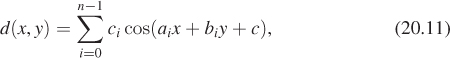
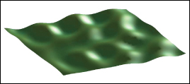
where the numbers ai, bi, and ci affect the orientation of the cosine waves, with ci displacing the ith wave along its direction of propagation and with ![]() determining its frequency. If the points (ai, bi) are chosen at random from an annular region in the plane given by r2 ≤ a2i +b2i ≤ R2, then the resultant waves will all have roughly similar periods, producing a result like that shown in Figure 20.14. Geoff Gardner [Gar85] called this a “poor man’s Fourier series,” because of the use of only n terms (many of his applications used something like n = 6 terms).
determining its frequency. If the points (ai, bi) are chosen at random from an annular region in the plane given by r2 ≤ a2i +b2i ≤ R2, then the resultant waves will all have roughly similar periods, producing a result like that shown in Figure 20.14. Geoff Gardner [Gar85] called this a “poor man’s Fourier series,” because of the use of only n terms (many of his applications used something like n = 6 terms).
By the way, Gardner also showed that this function could be used for other things; he used a three-dimensional version to represent the density of a cloud at a point (x, y, z), and the 2D version with thresholding to determine placement of vegetation in a scene: Anyplace where d was above some specified value, he placed a tree or a bush, generating remarkably plausible distributions.
20.8.2. Perlin Noise
Perlin [Per85, Per02b] took a different approach, aiming to directly produce “noise” whose Fourier transform was nonzero only within a modest band, or at least whose values outside that band were small, and where the noise values themselves were constrained to [−1, 1]. The main idea can be illustrated where the noise is a function of a single real parameter x. At each integer point we (a) want the value at that point to be 0, and (b) want the function to have some gradient, which for simplicity we choose to be 0, 1, or –1. If, at x = 4, we choose a gradient of +1, then we can build the function
which has the value 0 at x = 4, and the derivative +1 there. After picking gradients at each integer point, we get functions y1, y2, .... The idea is that on the interval 4 ≤ x ≤ 5, we can blend between y4(x) and y5(x) with a function that varies from 0 to 1 as x goes from 4 to 5. The fractional part of x, that is, x – 4, is such a function, which results in
Unfortunately, the resultant graph has sharp corners at integer values. To resolve this, we need a nicer interpolation. We will use the fractional part of x, xf = x – floor(x), as the argument to our blending function, namely,
which varies from a (0) = 0 to a (1) = 1, and has a′ (s) = 0 for s = 0, 1. The result is a second-order smooth interpolation between the successive linear functions. The result is shown in Figure 20.15.
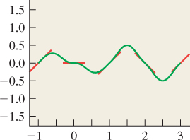
Figure 20.15: One-dimensional Perlin noise; the individual linear functions are shown as short red segments.
In practice, to create a larger version of Figure 20.15, we would generate, say, 20 random items from the set {–1, 0, 1} and use these as the gradient values at locations x = 0, 1, ..., 19. For values outside this range, we reduce mod 20. That produces a repeating pattern, but it is much faster than invoking a random number generator lots of times. Of course, one can choose any fixed number of gradients—20 or 200 or 2,000—to avoid repetition in practice.
Note that because the control points had unit spacing, the resultant spline curve had features that were spaced about a unit apart in general, and hence they had a Fourier transform that was concentrated at frequency one. This idea can be generalized to 2D and 3D. To generalize to three dimensions (2D is left as an exercise for you), we must select (3D) gradients at each integer point. Perlin recommends picking them from the set 12 vectors from the center of a cube to its edge midpoints, namely,
to avoid a kind of bias in which the gradient of the noise function ends up preferentially aligned with the coordinate axes. By appending a redundant row to this list, namely,
we end up with 16 vectors, which makes it easy to use bitwise arithmetic to select one of them.
Having assigned a gradient vector [u v w]T to the lattice point (i, j, k) we define a linear function
To find the noise value at a point (x, y, z), we let i0, j0, and k0 be the floor of x, y, and z, respectively, so that i0 ≤ x < i0 + 1, and similarly for y and z, and the eight corners of the grid cube containing (x, y, z) have coordinates (i0, j0, k0), (i0, j0, k0 + 1), (i0, j0+1, k0), ..., (i0+1, j0+1, k0+1). For each corner (i, j, k), we evaluate the linear function associated to that corner at the point (x, y, z) to get a value vi,j,k. We blend these values trilinearly using a(xf), a(yf), and a(zf). A direct but inefficient implementation is given in Listing 20.1 (the function a of Equation 20.14 must also be defined). Perlin [Per02a] provides an optimized implementation.
The result (in 2D) is shown in Figures 20.16 and 20.17.
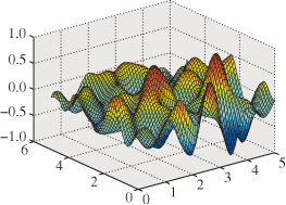
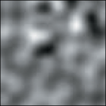
Figure 20.17: The same function, displayed as a grayscale image where – 1 is black and + 1 is white.
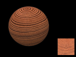
We can use 3D Perlin noise to create a radial displacement map on a sphere, while also coloring points by their displacement, to get a result like that shown in Figure 20.18.

Perlin [Per85] describes far more complex applications, allowing him to produce things like the marble texture in Figure 20.19.
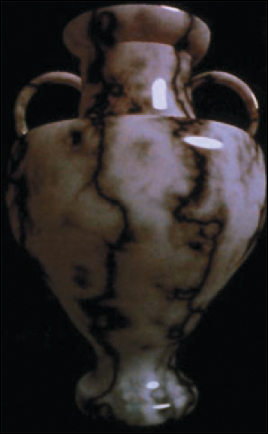
Figure 20.19: A marble vase with texture based on a complex combination of noise functions (Courtesy of Ken Perlin, © 1985 ACM, Inc. Reprinted by permission).
20.8.3. Reaction-Diffusion Textures
A third approach to texture synthesis is due to an idea by Turing [Tur52] about the formation of patterns like leopard spots or snake scales in nature. He conjectured that such patterns could arise from evolving concentrations of chemicals called morphogens. Typically, one starts with two morphogens, with concentrations randomly distributed across a surface. They evolve through a combination of two processes: diffusion, in which high concentrations of morphogens diffuse to fill in areas of low concentration, and reaction, in which the two morphogens combine chemically to either produce or consume one or both of the morphogens. If the presence of A promotes the production of B, but the presence of B promotes the consumption of A, for instance, interesting patterns can arise. The appearance of these patterns is governed by many things: the particular differential equation representing the change in morphogen A as a function of the concentrations of A and B, the rate (and direction) of diffusion of the morphogens, and the initial distribution of concentrations. Turing’s idea was that the steady-state concentration of one of the morphogens might control appearance so that, for example, a zebra’s skin would grow white hair where the concentration of morphogen A was small, but black hair where it was large.
Listing 20.1: An implementation of Perlin noise using a 256 × 256 × 256 cube as a tile.
1 grad[16][3] = (1, 1, 0), (-1, 1, 0), . . .
2
3 noise(x, y, z)
4 reduce x, y, z mod 256
5 i0 = floor(x); j0 = floor(y); k0 = floor(z);
6 xf = x - i0; yf = y - j0; zf = z - k0;
7 ax = a(xf) ; ay = a(yf) ; az = a(zf); // blending coeffs
8
9 for i = 0, 1; for j = 0, 1; for k = 0, 1
10 h[i][j][k] = hash(i0+i, j0 + j, k0 + k)
11 // a hash value between 0 and 15
12 g[i][j][k] = grad[h[i][j][k]]
13 v[i][j][k] = (x - (i0+i)) * g[i][j][k][0] +
14 (y - (j0+j)) * g[i][j][k][1] +
15 (z - (k0+k)) * g[i][j][k][2]
16
17 return blend3(v, ax, ay, az)
18
19 blend3(vals, ax, ay, az)
20 // linearly interpolate first in x, then y, then z.
21 x00 = interp(vals[0][0][0], vals[1][0][0], ax)
22 x01 = interp(vals[0][0][1], vals[1][0][1], ax)
23 x10 = interp(vals[0][1][0], vals[1][1][0], ax)
24 x11 = interp(vals[0][1][1], vals[1][1][1], ax)
25 xy0 = interp(x00, x10, ay)
26 xy1 = interp(x01, x11, ay)
27 xyz = interp(xy0, xy1, az)
28 return xyz
29
30 interp(v0, v1, a)
31 return (1-a) * v0 + a * v1
Turing lacked the computational power to perform simulations, but Turk [Tur91] and Kass and Witkin [WK91] took his ideas, extended them, and made it practical to run simulations to predict the steady-state concentrations resulting from some set of initial conditions, not only on the plane, but also on more general surfaces. Figure 20.20 shows some examples of the reaction-diffusion textures that they generated.
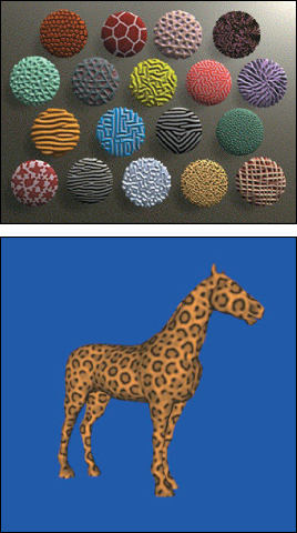
Figure 20.20: Reaction-diffusion textures. Top: Textures synthesized by Kass and Witkin. (Courtesy of Michael Kass, Pixar and Andrew Witkin, © 1991 ACM, Inc. Reprinted by permission). Bottom: Texture synthesized by Greg Turk. (Courtesy of Greg Turk, © 1991 ACM, Inc. Reprinted by permission.)
20.9. Data-Driven Texture Synthesis
As a final topic, we’ll briefly discuss two methods for generating new texture from old. The first of these is Ashikhmin’s texture synthesis algorithm [Ash01], which is based on ideas in papers by Efros and Leung [EL99] and Wei and Levoy [WL00], which in turn follow work of Popat and Picard [PP93]. The input for the algorithm is a texture image (e.g., a photograph of a brick wall) that’s called the source, and a size, n × k, of an image to be created. The output is an n× k image we’ll call the target; typically n× k is much larger than the size of the input image. The idea is that the target should look like it comes from “the same stuff as the source”; for example, like a photograph of a larger region of a brick wall. Figure 20.21 shows the idea. We fill in the target image row by row, moving left to right. At a typical point in the filling-in procedure, the blue-colored pixels have had their values determined and the yellow area is still to be processed. We select a small rectangle (2 × 3 in the figure) containing mostly known pixels, and one unknown (pink) pixel at the bottom right. (We’ll call this set of six pixels a template.) The goal is to determine a value for this last pixel, and then advance the template one step to the right.
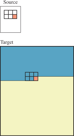
We take the five known pixels in the rectangle, and look in the source image for similarly shaped clusters that match these five known pixels. We then pick one with a good fit, and copy its sixth pixel into the appropriate spot in the target. We then move the template one step to the right, and proceed.
This description glosses over several important points, such as “How do we get started?” and “How do we move to a new row?” and “How do we find in the source image good-matching patches for the known template pixels without taking forever to do it?” One way to start is with random pixels from the source image filling the target. As we start at the upper left, finding a “match” for the first 5-pixel patch will be very difficult—we’ll have to be happy with a not-very-good result. But as we move forward, things gradually start to work better. To improve matters, we may want to run the algorithm several times, working top to bottom, bottom to top, left to right, right to left, etc., to clean up the edges.
As for finding good candidates as matching patches, one useful observation is that if you move the template one step to the right, a good candidate for filling in the next pixel is exactly one step to the right of the source pixel you just used (i.e., the algorithm’s very likely to favor copying whole rows of pixels). This can be generalized. For instance, right above the missing pixel is one that you filled in one row earlier. If we look at the corresponding source pixel, the one immediately below it is a good candidate for the missing pixel, too. In fact, the source locations of all five known template pixels similarly provide (with slight offsets) good candidate locations in which to find a source for the missing sixth pixel. The algorithm proceeds by picking a pixel from this candidate set. Occasionally (e.g., when a source pixel is near the edge of the image) this may not work, in which case we have to replace this candidate with another; there are many possible choices, and the details are not important.
The results are quite impressive. Figure 20.22 shows an example in which a few berries are used to synthesize many berries. The algorithm has another advantage: It’s possible to start with the target image partly filled in! We can declare in advance that we want certain pixels to have certain colors, and when the algorithm reaches these pixels, it finds them already “filled in” and leaves them unchanged. But their presence affects how well the subsequent patches fit with one another, and hence the synthesis of subsequent pixels. Figure 20.23 shows an example.
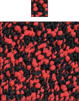
Figure 20.22: A tiny source image and a large image synthesized from it (Courtesy of Michael Ashikhmin, ©2001 ACM, Inc. Reprinted by permission.)

Figure 20.23: A source image, a hand-drawn “guide,” and the resulting synthesized image after five rounds of synthesis (Courtesy of Michael Ashikhmin, © 2001 ACM, Inc. Reprinted by permission.)
The end result of the synthesis process is that long diagonal strips from the source tend to be copied whole, in such a way that they match up with neighboring strips. Figure 20.24 shows this structure.
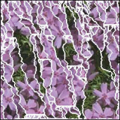
Figure 20.24: The striplike structure of a synthesized image. Coherent pixel regions are outlined in white. (Courtesy of Michael Ashikhmin, © 2001 ACM, Inc. Reprinted by permission.)
In this situation, a small square of the target image around some pixel (i, j) tends to match a small square in the source image around some pixel (i′, j′), although along the edges between strips this isn’t an exact match. If we compute vij = [i′ – i j′ – j]T, then we see that v tends to be locally constant as a function of i and j, precisely because of the approach that the algorithm takes, namely, using nearby pixels’ v-vectors as candidates for the v-vector of the pixel being synthesized.
This notion can be generalized: Given an image A and an image B, we can extract, for each pixel (i, j) of A, a p × p square P centered there, and look at every p × p patch in B to find one “closest” to P. We then find the center of this B-patch, (i′, j′), and set vij =] i′ – i j′ – j]T. The resultant collection of vectors is called a nearest-neighbor field (for patches of size p). Computing this field can be very slow, but if the images A and B are similar, the field tends to have the same kind of coherence exhibited by the results of the Ashikhmin algorithm: Neighboring pixels tend to have similar vectors. Barnes et al. [BSFG09] use this observation to develop an approach to computing the nearest-neighbor field (or a very close approximation) for two images very quickly.
While the resultant field might be used for texture synthesis if B is an example texture and A is a large image that has some structural resemblance to the texture in B, Barnes et al. actually describe a great many other computational photography applications based on it, such as the “image shuffling” shown in Figure 20.25, in which the user annotates a region (in this case, the person in the photo) and a place to which to move the region. A combination of the nearest-neighbor field computation and an expectation-maximization algorithm that seeks to fill in the hole (and adjust pixels near the moved region) in a way that makes the patch matching optimal produces the image in which the person appears to have moved within the photo.
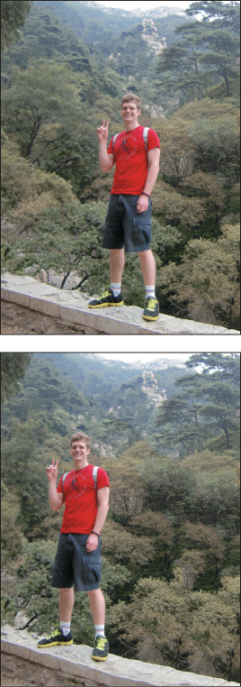
Figure 20.25: The man in the original image (a) is translated to the left in image (b). (Courtesy of Connelly Barnes)
20.10. Discussion and Further Reading
We’ve only touched on texture mapping here. Table 20.1 gives some hint of how powerful the method is, which should hardly be surprising, since at its essence, it’s “indirection” or “function evaluation,” both of which are at the very heart of computation.
With texture mapping, we’re (generally) altering parameters to a lighting computation. But in Chapter 31, we’ll see that what we actually want to compute for each sample in a rendering is an estimate of an integral, and the integrand has the general form of a lighting model. As we move from sample to sample, this integral varies. If the variation is not band-limited, we’ll get aliasing errors. But texture mapping makes certain that the individual parameters within the integrand are each band-limited, rather than the value of the integral. In other words, we’ve band-limited and then integrated, rather than integrated and then band-limited. Since these two operations do not generally commute, we’re producing potentially incorrect results. The degree to which they’re incorrect has not yet been thoroughly analyzed.
Although texture mapping is used in rendering, it’s also forced into service in more general computations. Both GL and DX shaders use texture maps as general-purpose RAM for storing arbitrary data structures. That is because the first graphics systems didn’t support random access memory or anything beyond primitive floating-point types. The practice of tricky uses of texture memory is losing currency with new hardware that supports arbitrary read and write operations, often using sophisticated abstractions. DirectCompute and CUDA shaders already just look like C programs with regard to memory access ...but they still have the useful API for texture fetches that implement mappings and filtering.
Texture synthesis is also a rich and active area of research, from ab initio methods like Cook and DeRose’s work on wavelet noise [CD05b], which generalizes Perlin noise, to work on detail hallucination, in which highly zoomed textures that would otherwise be blurry are enhanced with further detail that matches the neighboring texel values [SZT10, WWZ+07].
20.11. Exercises
![]() Exercise 20.1: In varying parameters to the Phong model, we’ve used texture mapping to adjust the incoming light, the outgoing light, and the diffuse and glossy constants. But we haven’t used it to modify the dot product. If we replace v · w = vTw with vTMw, where M is some symmetric matrix with positive eigenvalues, then the results computed by the Phong model will change depending on the orientation of the eigenvectors and the magnitudes of the eigenvalues. Apply this idea to the unit sphere. Writing M = VDVT where V contains the eigenvectors as columns, and D is a diagonal matrix with the eigenvalues on the diagonal, experiment with what happens when V = [t1 t2 n], where t1 and t2 are unit vectors tangent to the latitude and longitude lines, n is the surface normal, and D = Diag(s, t,1), where 0 < s, t ≤ 1. You should be able to achieve the general appearance of brushed metal if you use this altered inner product in the glossy part of the Phong model.
Exercise 20.1: In varying parameters to the Phong model, we’ve used texture mapping to adjust the incoming light, the outgoing light, and the diffuse and glossy constants. But we haven’t used it to modify the dot product. If we replace v · w = vTw with vTMw, where M is some symmetric matrix with positive eigenvalues, then the results computed by the Phong model will change depending on the orientation of the eigenvectors and the magnitudes of the eigenvalues. Apply this idea to the unit sphere. Writing M = VDVT where V contains the eigenvectors as columns, and D is a diagonal matrix with the eigenvalues on the diagonal, experiment with what happens when V = [t1 t2 n], where t1 and t2 are unit vectors tangent to the latitude and longitude lines, n is the surface normal, and D = Diag(s, t,1), where 0 < s, t ≤ 1. You should be able to achieve the general appearance of brushed metal if you use this altered inner product in the glossy part of the Phong model.
![]() Exercise 20.2: On the unit disk D in the plane, consider the vector field n(x, z) = S([–z 1 x]T). Show that there’s no function y = f(x, z) on D with the property that the normal vector to the graph of f at (x, f (x, z), z) is exactly n(x, z), that is, that n is not the normal field of any surface above D. Hint: Assume without loss of generality that f(1, 0) = 0. Now traverse the curve γ(t) = (cos t, 0, sin t),0 ≤ t ≤ 2π and see what you can say about the restriction of f to this curve.
Exercise 20.2: On the unit disk D in the plane, consider the vector field n(x, z) = S([–z 1 x]T). Show that there’s no function y = f(x, z) on D with the property that the normal vector to the graph of f at (x, f (x, z), z) is exactly n(x, z), that is, that n is not the normal field of any surface above D. Hint: Assume without loss of generality that f(1, 0) = 0. Now traverse the curve γ(t) = (cos t, 0, sin t),0 ≤ t ≤ 2π and see what you can say about the restriction of f to this curve.
Exercise 20.3: (a) Write a program to render a picture like the one shown in Figure 20.13. For the checkerboard itself, assuming 0 is black and 1 is white, make the light squares about 0.85 and the dark squares about 0.15, and be sure you can render a picture like the one shown.
(b) Figure out the size of the screen-space projection of a unit square at location (x,0, z) on the ground plane, either algebraically or by projecting the four corners and computing numerically. From this, determine the vertical and horizontal band limits as a function of x and z.
(c) The texture color at location (x, z) on the plane can be written as 0.5 + 0.35S(x)S(z), where S(x) = 1 if floor(x) is even, and –1 otherwise. With methods like those of Chapter 18, you can compute the Fourier series for S; it’s
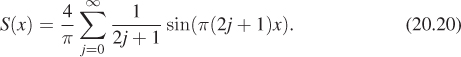
To band-limit this, you need only truncate the sum, and define
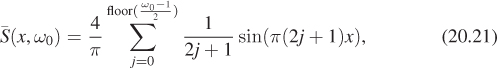
which removes all frequencies ω0 and above. Rerender your image using ![]() with an appropriate band limit, based on z, and compare aliasing in the rerendered image.
with an appropriate band limit, based on z, and compare aliasing in the rerendered image.
(d) The aliasing may still seem excessive to you, and the Gibbs phenomenon artifacts may also be annoying. Experiment with other approximations to a band-limited version of S, and with band limiting to a lower frequency than might seem necessary, and evaluate the results.
![]() (e) Truncating the series at the band limit (i.e., multiplying by a box in the frequency domain) is not the only way to remove high frequencies. Try using the Fejer kernel (i.e., multiplying by an appropriately dimensioned tent in the frequency domain) to see if you can get more satisfying results.
(e) Truncating the series at the band limit (i.e., multiplying by a box in the frequency domain) is not the only way to remove high frequencies. Try using the Fejer kernel (i.e., multiplying by an appropriately dimensioned tent in the frequency domain) to see if you can get more satisfying results.
Exercise 20.4: In two dimensions, imagine a parabolic mirror like the one shown in red in Figure 20.26, with the equation of the form ![]() . Rays (in green) coming from a semicircle of directions are reflected to become rays (in blue) parallel to the z-axis (and vice versa).
. Rays (in green) coming from a semicircle of directions are reflected to become rays (in blue) parallel to the z-axis (and vice versa).
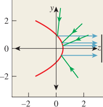
Figure 20.26: The red parabolic mirror reflects light from a semi-circle of directions onto a line segment.
(a) Show that the yz-vector n = [y, 1]T is normal to the red curve at the point ![]() .
.
(b) If light traveling in the direction [0 –1]T strikes the mirror at (y, z) and reflects, in what direction r does it leave? Write out your answer in terms of y and z.
(c) Show that at (±1, 0) the outgoing ray is in direction [±1 0]T.
(d) Show that incoming rays in direction [0 –1]T whose y-coordinate is between –1 and 1 become outgoing rays in all possible directions in the right half-plane.
(e) If you spin Figure 20.26 about the z-axis, the red curve generates a paraboloid. Show that in this situation, incoming rays in the direction [0 –1]T with starting points of the form (x, y,1), where x2 + y2 ≤ 1, produce all possible outgoing rays in the hemisphere of directions with z ≥ 0.
(f) If we take a second paraboloid defined by spinning ![]() , then arrows in direction [0 1]T, arriving from points of the form (x, y, –1), where x2 + y2 ≤ 1, reflect into outgoing rays in the opposite hemisphere of directions. These two reflections establish a correspondence between (1) two unit disks parallel to the xy-plane, and (2) two hemispheres of directions. Write out the inverse of this correspondence.
, then arrows in direction [0 1]T, arriving from points of the form (x, y, –1), where x2 + y2 ≤ 1, reflect into outgoing rays in the opposite hemisphere of directions. These two reflections establish a correspondence between (1) two unit disks parallel to the xy-plane, and (2) two hemispheres of directions. Write out the inverse of this correspondence.
(g) Explain how you can represent a texture map on the sphere (e.g., an irradiance map, or an environment map, etc.) by providing textures on two disks.
![]() (h) Estimate the largest value of the change of area for this “dual paraboloid” parameterization of the sphere to show that it uses texture memory quite effectively, even though π/4 of each texture image (the disk within the unit square) gets used for each half of the parameterization.
(h) Estimate the largest value of the change of area for this “dual paraboloid” parameterization of the sphere to show that it uses texture memory quite effectively, even though π/4 of each texture image (the disk within the unit square) gets used for each half of the parameterization.