
Chapter 14. Standard Approximations and Representations
14.1. Introduction
The real world contains too much detail for us to simulate it efficiently from first principles of physics and geometry. Mathematical models of the real world and the data structures and algorithms that implement them are always approximations. These approximations make graphics computationally tractable but introduce restrictions and error. The models and approximations are both geometric and algorithmic. For example, a ball is a simple geometric model of an orange. A simple computational model of light interaction might specify that the light passing through glass does not refract or lose energy.
In this chapter, we survey some pervasive approximations and their limitations. This chapter brings together a number of key assumptions about models and data structures for representing them that are implicit in the rest of the book and throughout graphics. It contains some of the engineering conventional wisdom and practical mathematical techniques accumulated over the past 50 years of computer graphics. It is what you need to know to apply your existing mathematics and computer science knowledge to computer graphics as it is practiced today. In order to quickly communicate a breadth of material, we’ll stay relatively shallow on details. Where there are deep implications of choosing a particular approximation, a later chapter on each particular topic will explain those implications with more nuance. To keep the text modular (and save you a lot of flipping), there is some duplication of ideas from both prior and succeeding chapters, and we’ve used some terms and units that have not yet been introduced, like steradians, but whose precise details don’t matter in a first reading at this stage.
The code samples in this chapter are based on the freely available OpenGL API (http://opengl.org) and G3D Innovation Engine library (http://g3d.sf.net). We recommend examining the details in the documentation for those or equivalent alternatives for further study of how these common approximations and representations manifest themselves in programming practice.
14.2. Evaluating Representations
In many cases, there are competing representations that have different properties. Which representation is best suited to a particular application depends on the goals of that application. Choosing the right representation for an application is a large part of the art of system design. Some factors to consider when evaluating a representation are
• Physical accuracy
• Perceived accuracy
• Design goals
• Space efficiency
• Time efficiency
• Implementation complexity
• Associated cost of content creation
Physical accuracy is the easiest property to measure objectively. We can use a calibrated camera to measure the energy reflected from a known scene and compare that to a rendering of the scene, for example, as is often done with the Cornell Box (see Figure 14.1).
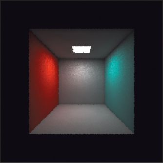
Figure 14.1: The Cornell box, a carefully measured five-sided, painted plywood box with a light source at the top, is used as a standard test model for rendering algorithms. Here it’s rendered by photon mapping with 1 million photons.
But physical accuracy is rarely the most important consideration in the creation of images. When the image is to be viewed by a human observer, errors that are imperceptible are less significant than those that are perceptible. So physical accuracy is the wrong metric for image quality. That’s also fortunate—regardless of how well we simulate a virtual scene, we are forced to accept huge errors from our displays. Today’s displays cannot reproduce the full intensity range of the real world and don’t create true 3D light fields into which you can focus your eyes.
Perceived accuracy is a better metric for quality, but it is hard to measure. There are many reasonable models that measure how a human observer will perceive a scene. These are used both for scientific analysis of new algorithms and directly as part of those algorithms—for example, video compression schemes frequently consider the perceptual error introduced by their compression. However, as discussed in Chapter 5, human perception is sensitive to the viewing environment, the task context, the image content, and of course, the particular human involved. So, while we can identify important perceptual trends, it is not possible to precisely quantify the reduction in perceived image quality at the level that we can quantify, say, a reduction in performance.
Even perceptual accuracy is not necessarily a good measure of image quality. A line drawing has little perceptual relationship to the hues and tones in a photograph, yet a good line drawing may be considered a higher-quality depiction of a scene than a poorly composed photograph, as shown in Figure 14.2. The model with best image quality is the one that best communicates the virtual scene to the viewer, in the style that the designer desires. This may be, for example, wireframe in a CAD program, painterly in an art piece, cartoony in a video game, or photorealistic for film. Often artists and designers intentionally simplify and deform geometric models, stylize lighting, and remove realism from rendering to better communicate their ideas. This kind of image quality is beyond objective measurement, which is one of the reasons that designing a graphics system is a subjective art as well as an engineering exercise.
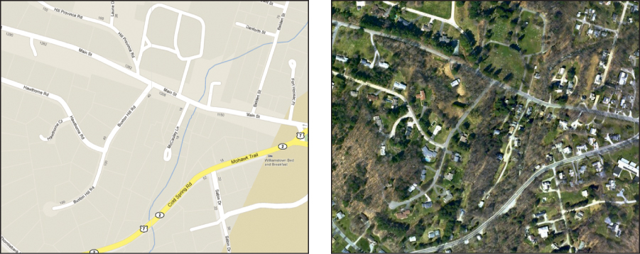
Figure 14.2: A map contains less information and detail than a satellite photograph, but presents its information in a way that better communicates the salient elements to a human viewer. This is evidence that capturing many aspects of reality is not always the most effective way to model a scene. (Credit: © 2012 Google - Map data © 2012 Cnes/Spot Image, DigitalGlobe, GeoEye, MassGIS, Commonwealth of Massachusetts EOEA, New York GIS, USDA Farm Service Agency)
Space and time efficiency and implementation complexity go beyond mathematical modeling and into implementation. We seek to actually implement the algorithms that we design and apply them to real problems. For real-time interactive rendering, efficiency is paramount. A low-quality animation that is interactive almost always leads to a better experience in a virtual world than a high-quality one with limited or high-latency interaction. The accessibility and viability of a system in the market is driven by price. The computational and memory requirements, and developer-time costs to build a system, must be balanced against the quality of the images produced.
14.2.1. The Value of Measurement
We can draw some lessons by considering measurements of image quality. Advances in graphics have largely focused on space and time efficiency and physical image quality, even though we claim that perceptual quality, fidelity to the designer’s vision, and implementation complexity are also important factors. This is likely because efficiency and physical quality are more amenable to objective measurement. They aren’t necessarily easier to optimize for, but the objective measurements allow quantitative optimization. So the first lesson is that if you want something to improve, find an objective way to quantify it. Today’s physical image quality is very high, and within some limits we can also achieve very good perceptual image quality. Feature films regularly contain completely computer-generated images that are indistinguishable from photographs, and even low-power mobile devices feature interactive 3D graphics. The second lesson is to make sure that you optimized for what you really wanted. (This is an instance of the Know Your Problem principle from Chapter 1!) Despite the many advances in image quality, the process of modeling, animating, and rendering scenes using either tools or code has not advanced as far as one might hope. Implementation complexity has skyrocketed over the past 50 years despite (and sometimes because of) graphics middleware libraries and standardization of certain algorithms. Progress has been very slow outside of photorealism, perhaps because the quality of nonphotorealistic renderings is evaluated subjectively. Computer graphics does not today empower the typical user with the expressive and communicative ability of an artist using natural media.
14.2.2. Legacy Models
Beware that in this chapter we describe both the representations that are preferred for current practice and some that are less frequently recommended today. Some of the older techniques make tradeoffs that one might not select intentionally if designing a system from a blank slate today. That can be because they were developed early in the history of computer graphics, before certain aspects were well understood. It can also be because they were developed for systems that lacked the resources to support a more sophisticated model.
We include techniques that we don’t recommend using for two reasons. First, this chapter describes what you need to know, not what you should do. Classic graphics papers contain great key ideas surrounded by modeling artifacts of their publication date. You need to understand the modeling artifacts to separate them from the key ideas. Graphics systems contain models needed to support legacy applications, such as Gouraud interpolation of per-vertex lighting in OpenGL. You will encounter and likely have to help maintain such systems and can’t abandon the past in practice.
Second, out-of-fashion ideas have a habit of returning in systems. As we discussed in this section, the best model for an application is rarely the most accurate—there are many factors to be considered. The relative costs of addressing these are highly dynamic. One source of change in cost is due to algorithmic discoveries. For example, the introduction of the fast Fourier transform, the rise of randomized algorithms, and the invention of shading languages changed the efficiency and implementation complexity of major graphics algorithms. Another source of change is hardware. Progress in computer graphics is intimately tied to the “constant factors” prescribed by the computers of the day, such as the ratio of memory size to clock speed or the power draw of a transistor relative to battery capacity. When technological or economic factors change these constants, the preferred models for software change with them. When real-time 3D computer graphics entered the consumer realm, it adopted models that the film industry had abandoned a decade earlier as too primitive. A film industry server farm could bring thousands of times more processing and memory to bear on a single frame than a consumer desktop or game console, so that industry faced a very different quality-to-performance tradeoff. More recently the introduction of 3D graphics in mobile form factors again resurrected some of the lower-quality approximations.
14.3. Real Numbers
An implicit assumption in most computer science is that we can represent real numbers with sufficient accuracy for our application in digital form. In graphics we often find ourselves dangerously close to the limit of available precision, and many errors are attributable to violations of that assumption. So, it is worth explicitly considering how we approximate real numbers before we build more interesting data structures that use them.
Fixed point, normalized fixed point, and floating point are the most pervasive approximations of real numbers employed in computer graphics programs. Each has finite precision, and error tends to increase as more operations are performed. When the precision is too low for a task, surprising errors can arise. These are often hard to debug because the algorithm may be correct—for real numbers—so mathematical tests will yield seemingly inconsistent results. For example, consider a physical simulation in which a ball approaches the ground. The simulator might compute that the ball must fall d meters to exactly contact the ground. It advances the ball d – 0.0001 meters, on the assumption that this will represent the state of the system immediately before the contact. However, after that transformation, a subsequent test reveals that the ball is in fact partly underneath the ground. This occurs because mathematically true statements, such as d = d – a + a (and especially, a = (a/b) * b), may not always hold for a particular approximation of real numbers. This is compounded by optimizing compilers. For example, a = b + c; e = a + d may yield a different result than e = b + c + d due to differing intermediate precision, and even if you write the former, your optimizing compiler may rewrite it as the latter. Perhaps the most commonly observed precision artifact today is self-shadowing “acne” caused by insufficient precision when computing the position of a point in the scene independently relative to the camera and to the light. When these give different results with an error in one direction, the point casts a shadow on itself. This manifests as dark parallel bands and dots across surfaces.
More exotic, and potentially more accurate, representations of real numbers are available than fixed and floating point. For example, rational numbers can be accurately encoded as the ratio of two bignums (i.e., dynamic bit-length integers). These rational numbers can be arbitrarily close approximations of real numbers, provided that we’re willing to spend the space and time to operate on them. Of course, we are seldom willing to pay that cost.
14.3.1. Fixed Point
Fixed-point representations specify a fixed number of binary digits and the location of a decimal point among those digits. They guarantee equal precision independent of magnitude. Thus, we can always bound the maximum error in the representation of a real number that lies within the representable range. Fixed point leads to fairly simple (i.e., low-cost) hardware implementation because the implementation of fixed-point operations is nearly identical to that of integer operations. The most basic form is exact integer representation, which almost always uses the two’s complement scheme for efficiently encoding negative values.
Fixed-point representations have four parameters: signed or unsigned, normalized or not, number of integer bits, and number of fractional bits. The latter two are often denoted using a decimal point. For example, “24.8 fixed point format” denotes a fixed-point representation that has 32 bits total, 24 of which are devoted to the integer portion and eight to the fractional portion.
An unsigned normalized b-bit fixed-point value corresponding to the integer 0 ≤ x ≤ 2b – 1 is interpreted as the real number x/(2b – 1), that is, on the range [0, 1]. A signed normalized fixed-point value has a range of [–1, 1]. Since direct mapping of the range [0, 2b – 1] to [–1, 1] would preclude an exact representation of 0, it is common to map the two lowest bit patterns to –1, thus sliding the number line slightly and making –1, 0, and 1 all exactly representable.
Normalized values are particularly important in computer graphics because we frequently need to represent unit vectors, dot products of unit vectors, and fractional reflectivities using compact storage.
A terse naming convention is desirable for expressing numeric types in a graphics program because there are frequently so many variations. One common convention for fixed point decorates int, or fix with prefixes and suffixes. In this convention, the prefix u denotes unsigned, the prefix n denotes normalized, and the suffix denotes the bit allocations using an underscore instead of a period. For example, uint8 is an 8-bit unsigned fixed-point number with range [0, 255] and ufix5_3 is an unsigned fixed-point number with 5 integer bits and 3 fractional bits on the range [0, 25 – 2–3] = [0, 31.875]. An even more terse variation of this in OpenGL is the use of I to represent non-normalized fixed point and an assumption of unsigned normalized representation. For example, GL_R8 indicates an 8-bit normalized value (unint8) on the range [0, 1] and GL_RI8 indicates an integer on the range [0, 255].
Some common fixed-point formats currently in use in hardware graphics are unsigned normalized 8-bit for reflectivity, normalized 8-bit for unit vectors, and 24.8 fixed point for 2D positions during rasterization. Fixed-point is infrequently used in modern software rendering. CPUs are not very efficient for most operations on fixed-point formats and software rendering today tends to focus on quality more than performance, so one less frequently seeks minimal data formats if they are inconvenient. The exception is software rasterization—24.8 format is used in hardware, not for performance but because fixed-point arithmetic is exact: a + b – b = a (so long as the intermediate results do not overflow), which is not the case for most floating-point a and b.
14.3.2. Floating Point
Floating-point representations allow the location of the decimal point to move—in some cases, far beyond the number of digits. Although the details of the commonly used IEEE 754 floating-point representations are slightly more complicated than scientific notation, the key ideas are similar. A number can be represented as a mantissa and an exponent; for example, a × 10b can be encoded by concatenating the bits of a and b, which are themselves integer or fixed-point numbers. In practice, the IEEE 754 representations allow explicit representation of concepts like “not a number” (e.g., 0/0) and positive and negative infinity. These could be, but rarely are, represented as specific bit patterns in fixed point. Floating point offers increased range or precision over fixed point at the same bit count; the catch is that it rarely offers both at the same time. The magnitude of the error in the approximation of a real number depends on the specific number; it tends to be larger for larger-magnitude numbers (see Figures 14.3, 14.4). This makes it complicated to bound the error in algorithms that use this representation. Floating point also tends to require more complicated circuits to implement.
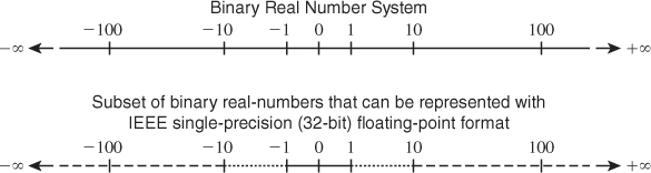
Figure 14.3: Subset of binary real numbers that can be represented with IEEE single-precision (32-bit) floating-point format. (Credit: Courtesy of Intel Corporation)
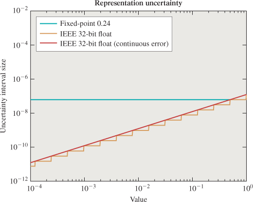
Figure 14.4: Distance between adjacent representable real numbers in 8.24-bit fixed point versus 32-bit floating point [AS06] over the range [10–4, 1). Floating-point representation accuracy varies with magnitude. ©2006 ACM, Inc. Included here by permission.
Both 32-bit and 64-bit floating-point numbers (sometimes called single-and double-precision) are common across all application domains. The 32-bit float is often preferred in graphics for space and time efficiency. Graphics also employs other floating-point sizes that are less common in other areas, such as 16-bit “half” precision and some very special-purpose sizes like 10-bit floating point (a.k.a. 7e3). Ten bits may seem like a strange size given that most architectures prefer power-of-two sizes for data types. In the context of a 3-vector storing XYZ or RGB values, three 10-bit values fit within a 32-bit word (the remaining two bits are then unused). Shared-exponent formats efficiently combine separate mantissas for each vector element with a single exponent [War94]. These are particularly useful for images, in which values may span a large range.
14.3.3. Buffers
The term of art, “buffer,” usually refers to a 2D rectangular array of “pixel” values in computer graphics; for example, an image ready for display or a map of the distance from the camera to the object seen at each pixel. Beware that in general computer science, a “buffer” is often a queue (and that sometimes a “2D vector” refers to a 2D array, not a geometric vector!); to avoid confusion, we never use the general computer science terminology in this book.
The color buffer holds the image shown on-screen in a graphics system. A reasonable representation might be a 2D array of pixel values, each of which stores three fields: red, green, and blue. Set aside the interpretation of those fields for the moment and consider the implementation details of this representation.
The fields should be small, that is, they should contain few bits. If the color buffer is too large then it might not fit in memory, so it is desirable to make each field as compact as possible without affecting the perceived quality of the final image. Furthermore, ordered access to the color buffer will be substantially faster if the working set fits into the processor’s memory cache. The smaller the fields, the more pixels that can fit in cache.
The size of each pixel in bits should be an integer multiple or fraction of the word size of the machine. If each pixel fits into a single word, then the memory system can make aligned read and write operations. Those are usually twice as fast as unaligned memory accesses, which must make two adjacent aligned accesses and synthesize the unaligned result. Aligned memory accesses are also required for hardware vector operations in which a set of adjacent memory locations are read and then processed in parallel. This might give another factor of 32 in performance on a vector architecture that has 32 lanes. If a pixel is larger than a word by an integer multiple, then multiple memory accesses are required to read it; however, vectorization and alignment are still preserved. If a pixel is smaller than a word by an integer multiple, then multiple pixels may be read with each aligned access, giving a kind of super-vectorization.
One common buffer format is shown in Figure 14.5. This figure shows a 3×3 buffer in the GL_R5G6B5 format. This is a normalized-fixed point format for 16-bit pixels. On a 64-bit computer, four of these pixels can be read or written with a single scalar instruction.
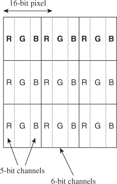
Figure 14.5: The GL_R5G6B5 buffer format packs three normalized fixed-point values representing red, green, blue, and coverage values, each on [0, 1], into every 16-bit pixel. The red and blue channels each receive five bits. Because 16 is not evenly divisible by three, the “extra” bit is (mostly arbitrarily) assigned to the green channel.
Five bits per channel is not much considering that the human eye can distinguish hundreds of shades of gray. Eight bits per channel enable 256 monochrome shades. But three 8-bit channels consume 24 bits, and most memory systems are built on power-of-two word sizes. One solution is to round up to a 32-bit pixel and simply leave the last eight bits of each pixel unused. This is a common practice beyond graphics—compilers often align the fields of data structures with such unused bits to enable efficient aligned memory access. However, it is also common in graphics to store some other value in the available space. For example, the common GL_RGBA8 format stores three 8-bit normalized fixed-point color channels and an additional 8-bit normalized fixed-point value called α (or “alpha,” represented by an “A”) in the remaining space (see Figure 14.6). This value might represent coverage, where α = 0 is a pixel that the viewer should be able to see through and α = 1 is a completely opaque pixel.
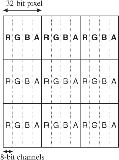
Figure 14.6: The GL_RGBA8 buffer format packs three 8-bit normalized fixed-point values representing red, green, blue, and coverage values, each on [0, 1], into every 32-bit pixel. This format allows efficient, word-aligned access to an entire pixel for a memory system with 32-bit words. A 64-bit system might fetch two pixels at once and mask off the unneeded bits—although if processing multiple pixels of an image in parallel, both pixels likely need to be read anyway.
Obviously, on most displays one cannot see through the display itself when a color buffer pixel has α = 0; however, the color buffer may not be intended for direct display. Perhaps we are rendering an image that will itself be composited into another image. When writing this book, we prepared horizontal and vertical grid lines of Figure 14.5 as an image in a drawing program and left the pixels that appear “white” on the page as “transparent.” The drawing program stored those values with α = 0. We then pasted the grid over the text labels “R,” “G,” etc. Because the color buffer from the grid image indicated that the interior of the grid cells had no coverage, the text labels showed through, rather than being covered with white squares. We return more extensively to coverage and transmission in Section 14.10.2.
The compositing example is one of many cases where a buffer is intended as input for an algorithm rather than for direct display to a human as an image, and α is only one of many common quantities found in buffers that has no direct visible representation. For example, it is common to store “depth” in a buffer that corresponds 1:1 to the color buffer. A depth buffer stores some value that maps monotonically to distance from the center of projection to the surface seen at a pixel (we motivate and show how to implement and use a depth buffer in Chapter 15, and evaluate variations on the method and alternatives extensively in Chapter 36 and Section 36.3 in particular).
Another example is a stencil buffer, which stores arbitrary bit codes that are frequently used to mask out parts of an image during processing in the way that a physical stencil (see Figure 14.7) does during painting.
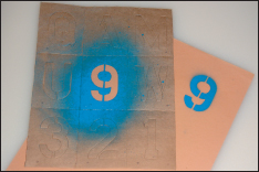
Figure 14.7: A real “stencil” is a piece of paper with a shape cut out of it. The stencil is placed against a surface and then painted over. When the stencil is removed, the surface is only painted where the holes were. A computer graphics stencil is a buffer of data that provides similar functionality.
Stencil buffers typically use very few bits, so it is common to pack them into some other buffer. For example, Figure 14.8 shows a 3×3 combined depth-and-stencil buffer in the GL_DEPTH24STENCIL8 format.
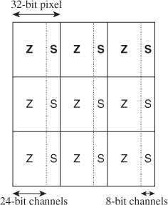
Figure 14.8: The GL_DEPTH24 STENCIL8 buffer format encodes a 24-bit normalized fixed point “depth” value with eight stencil bits used for arbitrary masking operations.
A framebuffer1 is an array of buffers with the same dimensions. For example, a framebuffer might contain a GL_RGBA8 color buffer and a GL_DEPTH24STENCIL8 depth-and-stencil buffer. The individual buffers act as parallel arrays of fields at each pixel. A program might have multiple framebuffers with many-to-many relationships to the individual buffers.
1. The framebuffer is an abstraction of an older idea called the “frame buffer,” which was a buffer that held the pixels of the frame. The modern parallel-rendering term is “framebuffer” as a nod to history, but note that it is no longer an actual buffer. It stores the other buffers (depth, color, stencil, etc.). Old “frame buffers” stored multiple “planes” or kinds of values at each pixel, but they often stored these values in the pixel, using an array-of-structs model. Parallel processors don’t work as well with an array of structs, so a struct of arrays became preferred for the modern “framebuffer.”
Why create the framebuffer level of abstraction at all? In the previous example, instead of two buffers, one storing four channels and one with two, why not simply store a single six-channel buffer? One reason for framebuffers is the many-to-many relationship. Consider a 3D modeling program that shows two views of the same object with a common camera but different rendering styles. The left view is wireframe with hidden lines removed, which allows the artist to see the tessellation of the meshes involved. The right view has full, realistic shading. These images can be rendered with two framebuffers. The framebuffers share a single depth buffer but have different color buffers.
Another reason for framebuffers is that the semantic model of channels of specific-bit widths might not match the true implementation, even though it was motivated by implementation details. For example, depth buffers are highly amenable to lossless spatial compression because of how they are computed from continuous surfaces and the spatial-coherence characteristics of typically rendered scenes. Thus, a compressed representation of the depth buffer might take significantly less space (and correspondingly take less time to access because doing so consumes less memory bandwidth) than a naive representation. Yet the compressed representation in this case still maintains the full precision required by the semantic buffer format requested through an API. Unsurprisingly given these observations, it is common practice to store depth buffers in compressed form but present them with the semantics of uncompressed buffers [HAM06]. Taking advantage of this compressibility, especially using dedicated circuitry in a hardware renderer, requires storing the depth values separately from the other channels. Thus, the framebuffer/color buffer distinction steers the high-level system toward an efficient low-level implementation while abstracting the details of that implementation.
14.4. Building Blocks of Ray Optics
In the real world, light sources emit photons. These scatter through the world and interact with matter. Some scatter from matter, through an aperture, and then onto a sensor. The aperture may be the iris of a human observer and the sensor that person’s retina. Alternatively, the aperture may be at the lens of a camera and the sensor the film or CCD that captures the image. Photorealistic rendering models these systems, from emitter to sensor. It depends on five other categories of models:
1. Light
2. Light emitters
3. Light transport
4. Matter
5. Sensors and their imaging apertures and optics (e.g., cameras and eyes)
We now explore the concepts of each category and some high-level aspects that can be abstracted to conserve space, time, and implementation complexity. Later in the chapter we return to specific common models within each category. We must defer that until later because the models interact, so it is important to understand all before refining any.
Although the first few sections of this chapter have covered a great many details, there is a high-level message as well, one that we summarize in a principle we apply throughout the remainder of the chapter:
![]() The High-Level Design Principle
The High-Level Design Principle
Start from the broadest possible view. Elements of a graphics system don’t separate as cleanly as we might like; you can’t design the ideal representation for an emitter without considering its impact on light transport. Investing time at the high level lets us avoid the drawbacks of committing, even if it defers gratification.
14.4.1. Light
14.4.1.1. The Visible Spectrum
The energy of real light is transported by photons. Each photon is a quantized amount of energy, so a powerful beam of light contains more photons than a weak beam with the same spectrum, not more powerful photons. The exact amount of energy per photon determines the frequency of the corresponding electromagnetic wave; we perceive it as color. Low-frequency photons appear red to us and high-frequency ones appear blue, with the entire rainbow spectrum in between (see Figure 14.9). “Low” and “high” here are used relative to the visible spectrum. There are photons whose frequencies are outside the visible spectrum, but those can’t directly affect rendering, so they are almost always ignored.
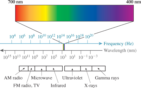
Figure 14.9: The visible spectrum is part of the full electromagnetic spectrum. The color of light that we perceive from an electromagnetic wave is determined by its frequency. The relationship between frequency and wavelength is determined by the medium through which the wave is propagating. (Courtesy of Leonard McMillan)
The human visual system perceives light containing a mixture of photons of different frequencies as a color somewhere between those created by the individual photons. For example, a mixture of “red” and “green” photons appears yellow, and is mostly indistinguishable from pure “yellow” photons. This aliasing (i.e., the substitutability of one item for another) is fortunate. It allows displays to create the appearance of many colors using only three relatively narrow frequency bands. Digital cameras also rely on this principle—because the image will be displayed using three frequencies, they only need to measure three.2 Most significantly for our purposes, almost all 3D rendering treats photons as belonging to three distinct frequencies (or bands of frequencies), corresponding to red, green, and blue. This includes film and games; some niche predictive rendering does simulate more spectral samples. We’ll informally refer to rendering with three “frequencies,” when what we really mean is “rendering with three frequency bands,” Using only three frequencies in simulation minimizes both the space and time cost of rendering algorithms. It creates two limitations. The first is that certain phenomena are impossible to simulate with only three frequencies. For example, the colors of clothing often appear different under fluorescent light and sunlight, even though these light sources may themselves appear fairly similar. This is partly because fluorescent bulbs produce white light by mixing a set of narrow frequency bands, while photons from the sun span the entire visible spectrum. The second limitation of using only three frequencies is that renderers, cameras, and displays rarely use the same three frequencies. Each system is able to create the perception of a slightly different space of colors, called a gamut. Some colors may simply be outside the gamut of a particular device and lost during capture or display. This also means that the input and output image data for a renderer must be adjusted based on the color profile of the device. Today most devices automatically convert to and from a standard color profile, called sRGB, so color shifts are minimized on such devices but gamut remains a problem.
2. This is not strictly true; Chapter 28 explains why.
![]() The Noncommutativity Principle
The Noncommutativity Principle
The order of operations often matters in graphics. Swapping the order of operations can introduce both efficiencies in computations and errors in results. You should be sure that you know when you’re doing so.
14.4.1.2. Propagation
The speed of propagation of a photon is determined by a material. In a vacuum, it is about c = 3 × 10⁸ m/s, which is therefore called the speed of light. The index of refraction of a material is the ratio of the speed of light in a vacuum to the rate s of propagation in that material:
For everyday materials, s < c, so η ≥ 1 (e.g., household glass has η ≈ 1.5). The exact propagation speed and index of refraction depend on the wavelength of the photon, but the variation is small within the visible spectrum, so it is common to use a single constant for all wavelengths. The primary limitation of this approximation is that the angle of refraction at the interface to a transmissive material is constant for all wavelengths, when it should in fact vary slightly. Effects like rainbows and the spectrum seen from a prism cannot be rendered under this approximation—but when simulating only three wavelengths, rainbows would have only three colors anyway.
Beware that it is common in graphics to refer to the wavelength λ of a photon, which is related to temporal frequency3 f by
3. Waves have a temporal frequency measured in 1/s (i.e., Hz) and a spatial frequency measured in 1/m. The spatial frequency of a photon is necessarily 1/λ and is rarely used in graphics because it varies with the speed of propagation.
Because the speed of propagation changes when a stream of photons enters a different medium, the wavelength also changes. Yet in graphics we assume that each of our spectral samples is fixed independent of the speed of propagation, so frequency is really what is meant in most cases.
Photons propagate along rays within a volume that has a uniform index of refraction, even if the material in that volume is chemically or structurally inhomogeneous. Photons are also selectively absorbed, which is why the world looks darker when seen through a thick pane of glass. At the boundary between volumes with different indices of refraction, light scatters by reflecting and refracting in complex ways determined by the microscopic geometry and chemistry of the material. Chapter 26 describes the physics and measurement of light in detail, and Chapter 27 discusses scattering.
14.4.1.3. Units
Photons transport energy, which is measured in joules. They move immensely fast compared to a human timescale, so renderers simulate the steady state observed under continuous streams of photons. The power of a stream of photons is the rate of energy delivery per unit time, measured in watts. You are familiar with appliance labels that measure the consumption in watts and kilowatts. Common household lighting solutions today convert 4% to 10% of the power they consume into visible light, so a typical “100 W” incandescent lightbulb emits at best 10 W of visible light, with 4 W being a more typical value.
In addition to measuring power in watts, there are two other measurements of light that appear frequently in rendering. The first is the power per unit area entering or leaving a surface, in units of W/m2. This is called irradiance or radiosity and is especially useful for measuring the light transported between matte surfaces like painted walls. The second is the power per unit area per unit solid angle, measured4 in W/(m2 sr), which is called radiance. It is conserved along a ray in a homogeneous medium. It is the quantity transported between two points on different surfaces, and from a point on a surface to a sample location on the image plane.
4. The unit “sr” is “steradians,” a measure of the size of a region on the unit sphere, described in more detail in Section 14.11.1.
14.4.1.4. Implementation
It is common practice to represent all of these quantities using a generic 3-vector class (e.g., as done in the GLSL and HLSL APIs), although in general-purpose languages it is frequently considered better practice to at least name the fields based on their frequency, as shown in Listing 14.1.
Listing 14.1: A general class for recording quantities sampled at three visible frequencies.
1 class Color3 {
2 public:
3 /** Magnitude near 650 THz ("red"), either at a single
4 frequency or representing a broad range centered at
5 650 THz, depending on the usage context. 650 THz
6 photons have a wavelength of about 450 nm in air. */
7 float r;
8
9 /** Near 550 THz ("green"); about 500 nm in air. */
10 float g;
11
12 /** Near 450 THz ("blue"); about 650 nm in air. */
13 float b;
14
15 Color3() : r(0), g(0), b(0) {}
16 Color3(float r, float g, float b) : r(r), g(g), b(b);
17 Color3 operator*(float s) const {
18 return Color3(s * r, s * g, s * b);
19 }
20 ...
21 };
One could use the type system to help track units by creating distinct classes for power, radiance, etc. However, it is often convenient to reduce the complexity of the types in a program by simply aliasing these to the common “color”5 class, as shown, for example, in Listing 14.2.
5. We discuss why color is not a quantifiable phenomenon in Chapter 28; here we use the term in a nontechnical fashion that is casual jargon in the field.
Listing 14.2: Aliases of Color3 with unit semantics.
1 typedef Color3 Power3;
2 typedef Color3 Radiosity3;
3 typedef Color3 Radiance3;
4 typedef Color3 Biradiance3;
Because bandwidth and total storage space are often limited resources, it is common to employ the fewest bits practical for your needs for each frequency-varying quantity. One implementation strategy is to parameterize the class, as shown in Listing 14.3.
Listing 14.3: A templated Color class and instantiations.
1 template<class T>
2 class Color3 {
3 public:
4 T r, g, b;
5
6 Color3() : r(0), g(0), b(0) {}
7 ...
8 };
9
10 /** Matches GL_RGB8 format */
11 typedef Color3<unint8> Color3un8;
12
13 /** Matches GL_RGB32F format */
14 typedef Color3<float> Color3f32;
15
16 /** Matches GL_RGB16I format */
17 typedef Color3<unsigned short> Color3ui16;
14.4.2. Emitters
Emitters are fairly straightforward to model accurately. They create and cast photons into the scene. The photons have locations, propagation directions, and frequencies (i.e., “colors”), and are emitted at some rate. Given probability distributions for those parameters, we can generate many representative photons and trace them through the scene. We say “representative” because real images are formed by trillions of photons, yet graphics applications can typically estimate the image very well from only a few million photons, so each graphics photon represents many real ones. Today’s computers and rendering algorithms can execute a simulation in this model for rendering images in a few minutes. The emission itself isn’t particularly expensive. Instead, the later steps of the tracing consume most of the processing time because each representative photon must be handled individually, and the interaction of millions of photons with millions or billions of polygons can be complicated.
To render even faster, we can simplify the emission model so that an aggregate of photons along a light ray can be considered by the later light transport steps. This is a common approximation for real-time rendering. The simplified models tend to fix the origin for all photons from an emitter at a single point. Doing so allows algorithms to amortize the cost of processing light rays from an emitter over the large number of light rays that share a single origin. As we said earlier, it is common practice to consider a small number of frequencies, to simplify the spectral representation, and to treat photons in the aggregate by measuring the average rate of energy emitted at each of those frequencies. Three frequencies loosely corresponding to “red,” “green,” and “blue” are almost always chosen to represent the visible spectrum, where each represents a weighted sum of the spectral values over an interval of the true spectrum, but is treated during simulation as a point sample, say, at the center of the interval. For an example of a more refined model, Pharr and Humphreys [PH10] describe a renderer with a nice abstraction of spectral curves.
14.4.3. Light Transport
In computer graphics, light transport is almost always modeled by (steady-state) ray optics on uncollimated, unpolarized light. This substantially simplifies the simulation by neglecting phase and polarization. In this model, photons propagate along straight lines through empty space. They do not interfere with one another, and their energy contribution simply sums. Under this simplification and with a discrete set of frequency samples, a geometric ray and a radiance vector (indicating radiance in the red, green, and blue portions of the spectrum) are sufficient to represent a stream of photons.
We’ll see in Chapter 27 that ignoring photon interference and polarization to simplify the representation of light energy is what forces us to complicate our representation of matter. For example, glossy and perfect reflection arises from the interference of nearly parallel streams of photons. This interference does not arise under ray optics, so we must introduce specific terms (such as Fresnel terms) to materials to model the same phenomena. One could use a richer model of light and a simpler model of a surface to produce the same image. However, a simple model of matter is not necessarily one that is easy to describe in terms of macroscopic phenomena, either for specification or for digital representation. Representing and modeling a brick as a rough, reddish slab of dried clay is both intuitive and compact. Representing it as a collection of 1026 or so molecules of varying composition is unwieldy at best.
14.4.4. Matter
There are many models of matter in graphics. The simplest is that matter is geometry that scatters light, and further, that this light scattering takes place only at the surfaces of opaque objects, ignoring the very small interactions of photons with air over short distances and any subsurface interaction effects. The surface scattering model builds on these assumptions by modeling only the surfaces of opaque objects. This reduces the complexity of a scene substantially. For example, a computer graphics car might have no engine, and a computer graphics house might be only a façade. Only the parts of objects that can interact with light need to be modeled. Of course, this approach poorly represents matter with deep interaction, such as skin and fog, and is only sufficient for rendering. To animate objects, for instance, we need to know properties such as joint locations and masses.
A consequence of computer graphics relying on complex models of matter is that different models are often employed for surface detail at different scales. Supporting different models and ways of combining them at intermediate scales complicates a graphics system. However, it also yields great efficiencies and matches our everyday perception. For example, from 100 meters, you might observe that a fir tree is similar to a green cone. From ten meters, individual branches are visible. From one meter, you can see separate needles. At one centimeter, small bumps and details on the needles and branches emerge. With a light microscope you can see individual cells, and with an electron microscope you can see molecule-scale detail. For this chapter, we consider details to be large-scale if their impact on the silhouette can be observed from about one meter, medium scale if they are smaller than that but observable by the naked eye at some scale, and small-scale if they are not observable by the naked eye.
14.4.5. Cameras
Lenses and sensors (the components of eyes and cameras) are complicated. This is true whether they have biological or mechanical origins. From a photographer’s perspective, the ideal lens would focus all light from a point that is “in focus” onto a single point on the imager (the sensing surface of the sensor) regardless of the frequency of light or the location on the imager. Real lenses have imperfect geometry that distorts the image slightly over the image plane and causes darkening near the edges, an effect known as vignetting (see Figure 14.10). They also necessarily focus different frequencies differently, creating an artifact called chromatic aberration (see Figure 14.11; see also Chapter 26). Camera manufacturers compensate for these limitations by combining multiple lenses. Unfortunately, these compound lenses absorb more light, create internal reflections, and can diffuse the focus. We perceive the reflections as lens flare—a series of iris shapes in line with the light source overlaid on the image, as seen in Figure 14.12. We perceive slightly diffused focus as bloom, where very bright objects appear defocused. Real film has a complex nonlinear response to light, and has grain that arises from the manufacturing process. Digital imagers are sensitive to thermal noise and have small divisions between pixels.
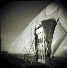
Figure 14.10: The darkening of this photograph near the edges is called vignetting. (Credit: Swanson Tennis Center at Gustavus Adolphus College by Joe Lencioni, shiftingpixel.com)

Figure 14.11: The rainbowlike edges on the objects in this photograph are caused by chromatic aberration in the camera’s lens. Different frequencies of light refract at different angles, so the resultant colors shift in the image plane. High-quality cameras use multiple lenses to compensate for this effect. (Credit: Corepics VOF/Shutterstock)
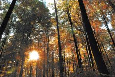
Figure 14.12: The streaks from the sun and apparently translucent-colored polygons and circles along a line through the sun in this photograph are a lens flare created by the intense light reflecting within the multiple lenses of the camera objective. Light from all parts of the scene makes these reflections, but most are so dim compared to the sun that their impact on the image is immeasurable. (Credit: Spiber/Shutterstock)
Since the simple model of a lens as an ideal focusing device and a sensor as an ideal photon measurement device yields higher image quality than a realistic camera model, there is little reason to use a more realistic model. Because lens flare, film grain, bloom, and vignetting are recognized as elements of realism from films, those are sometimes modeled using a post-processing pass. There is no need to model the true camera optics to produce these effects, since they are being added for aesthetics and not realism. Note that this arises purely from camera culture—except for bloom, none of these effects are observed by the naked eye.
14.5. Large-Scale Object Geometry
This section describes common models of object surfaces. Many rendering algorithms interact only with those surfaces. Some interact with the interior of objects, whose boundaries can still be represented by these methods. Section 14.7 briefly describes some representations for objects with substantial internal detail.
Some objects are modeled as thin, two-sided surfaces. A butterfly’s wing and a thin sheet of cloth might be modeled this way. These models have zero volume—there is no “inside” to the model. More commonly, objects have volume, but the details inside are irrelevant. For an opaque object with volume, the surface typically represents the side seen from the outside of the object. There is no need to model the inner surface or interior details, because they are never seen (see Chapter 36). To eliminate the inner side of the skin of an object, polygons have an orientation. The front face of a polygon is the side indicated to face outward and the back face is the side that faces inward. A process called backface culling eliminates the inward-facing side of each polygon early in the rendering process. Of course, this model is revealed as a single-sided, hollow skin should the viewer ever enter the model and attempt to observe the inside, as you saw in Chapter 6. This happens occasionally in games due to programming errors. Because there is no detail inside such an object and the back faces of the outer skin are not visible, in this case the entire model seems to disappear from view once the viewpoint passes through its surface.
Translucent objects naturally reveal their interior and back faces, so they require special consideration. They are often modeled either as a translucent, two-sided shell, or as two surfaces: an outside-to-inside interface and an inside-to-outside interface. The latter model is necessary for simulating refraction, which is sensitive to whether light rays are entering or leaving the object.
Surface and object geometry is useful for more than rendering. Intersections of geometry are used for modeling and simulation. For example, we can model an ice-cream cone with a bite taken out as a cone topped by a hemisphere ...with some smaller balls subtracted from the hemisphere. Simulation systems often use collision proxy geometry that is substantially simpler than the geometry that is rendered. A character modeled as a mesh of 1 million polygons might be simulated as a collection of 20 ellipsoids. Detecting the intersection of a small number of ellipsoids is more computationally efficient than detecting the intersection of a large number of polygons, yet the resultant perceived inaccuracy of simulation may be small.
14.5.1. Meshes
14.5.1.1. Indexed Triangle Meshes
Indexed triangle meshes (see Chapter 8) are a pervasive surface representation in graphics. The minimal representation is an array of vertices and a list of indices expressing connectivity. There are three common base schemes for the index list. These are called triangle list (or sometimes soup), triangle strip, and triangle fan representations. Figures 14.13 through 14.15 describe each in the context of counterclockwise triangle winding and 0-based indexing for a list describing n > 0 triangles.
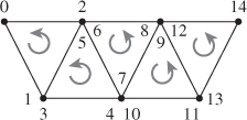
Figure 14.13: A triangle list, also known as a triangle soup, contains 3n indices. List elements 3t, 3t + 1, and 3t + 2 are the ordered indices of triangle t.
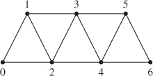
Figure 14.14: A triangle strip contains n + 2 indices. The ordered indices of triangle t are given as follows. For even t, use list elements t, t + 2, t + 1. For odd t, use list elements t, t + 1, t + 2.
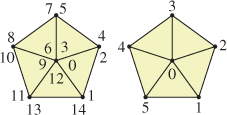
Figure 14.15: A triangle soup pentagon on the left, and the more efficient triangle fan model on the right. A triangle fan contains n + 2 indices. List elements 0, t + 1, t + 2 are the ordered indices of triangle t (with indices taken mod n + 2).
14.5.1.2. Alternative Mesh Structures
For each representation there is a corresponding nonindexed representation as a list whose element j is vertex[index[j]] from the indexed representation. Such nonindexed representations are occasionally useful for streaming large meshes that would not fit in core memory through a system. Because they duplicate storage of vertices (which are frequently much larger than indices), these representations are out of favor for moderate-sized models.
One can also construct quadrilateral or higher-order polygon meshes following comparable schemes. However, triangles have several advantages because they are the 2D simplex: Triangles are always planar, define an unambiguous barycentric interpolation scheme, never self-intersect, and are irreducible to simpler polygons. These properties also make them slightly easier to rasterize, ray trace, and sample than higher-order polygons. Of course, for data such as city architecture that is naturally modeled by quadrilaterals, a triangle mesh representation increases storage space without increasing model resolution.
14.5.1.3. Adjacency Information
Some algorithms require efficient computation of adjacency information between faces, edges, and vertices on a mesh. For example, consider the problem of rendering the contour of a convex mesh for a line-art program. Each edge is drawn only if it is on the contour. An edge lies between two faces. It is on the contour if exactly one face is oriented toward the viewer. We can make this determination more quickly if we augment the minimal indexed mesh with additional information describing faces, edges, and adjacency. Under that representation, we might directly iterate over edges (instead of triangles) and expect constant-time access to the two faces adjacent to each edge.
Adjacency information depends only on topology, so it may be precomputed for an animated mesh so long as the mesh does not “tear apart” under animation. Listing 14.4 gives a possible representation for a mesh with full adjacency information. In the listing, all the integers in the Vertex, Edge, and Face classes are indices into the arrays at the bottom of the class definition. Because faces are oriented, the order of elements matters in their vertices index arrays. This is the modern array-based equivalent of a classic mesh data structure called the winged edge polyhedral representation [Bau72] (see Chapter 8).
There are several ways to encode the edge information within these data structures. One is to consider the directed half-edges that each exist in one face. A true edge that is not on the boundary of the edge would then be a pair of half-edges. The half-edge representation offers the advantage of retaining orientation information when it is reached by following an index from a face. It has the disadvantage of storing redundant information for all the edges with two adjacent faces. A common trick obfuscates the code a bit by eliminating this storage overhead. The trick is to store only one half-edge for each mesh edge, and to index from a face using two’s complement when the half-edge is oriented opposite the direction that it should appear in that face. The two’s complement of a non-negative index e (written ~e in C-like languages) is guaranteed to be a negative number, so indices of oppositely directed edges are easy to identify. The two’s complement operator is efficient on most architectures, so it incurs little overhead. Each edge then uses the same trick to encode the indices of the adjacent faces, indicating whether that half-edge or its oppositely directed mate actually appears in the face.
Listing 14.4: Sample mesh representation with full adjacency information.
1 struct Mesh {
2 enum NO_FACE = MAX_INT;
3
4 struct Vertex {
5 Point3 location;
6 std::vector<int> edges;
7 std::vector<int> faces;
8 };
9
10 struct Edge {
11 int vertices[2];
12 /* May be NO_FACE if this edge is on a boundary. */
13 int faces[2];
14 };
15
16 struct Face {
17 int vertices[3];
18 int edges[3];
19 };
20
21 std::vector<int> index;
22 std::vector<Vertex> vertex;
23 std::vector<Edge> edge;
24 std::vector<Face> face;
25 };
14.5.1.4. Per-Vertex Properties
It is common to label the vertices of a mesh with additional information. Common rendering properties include shading normals, texture coordinates, and tangent-space bases.
A polygonal approximation of a curved surface appears faceted. The perception of faceting can be greatly reduced by shading the surface as if it were curved, that is, by shading the points indicated by the surface geometry, but altering the orientation of their tangent plane during illumination computations, as you saw in Chapter 6. It is common to model the orientation by specifying the desired surface normal at each vertex and interpolating between those normals within the surface of each polygon.
Texture coordinates are the additional points or vectors specified at each vertex to create a mapping from the surface of the model to a texture space that defines material properties, such as reflectance spectrum (“color”). Mapping from the surface to a 2D square using 2D points is perhaps the most common, but mappings to 1D spaces, 3D volumetric spaces, and the 2D surface of a 3D sphere are also common; Chapter 20 discusses this in detail. The last is sometimes called cube mapping, sphere mapping, or environment mapping depending on the specific parameterization and application.
A tangent space is just a plane that is tangent to a surface at a point. A mesh’s tangent space is undefined at edges and vertices. However, when the mesh has vertex normals there is an implied tangent space (the plane perpendicular to the vertex normal) at each vertex. The interpolated normals across faces (and edges) similarly imply tangent spaces at every point on the mesh. Many rendering algorithms depend on the orientation of a surface within its tangent plane. For example, a hair-rendering algorithm that models the hair as a solid “helmet” needs to know the orientation of the hair (i.e., which way it was combed) at every point on the surface. A tangent-space basis is one way to specify the orientation; it is simply a pair of linearly independent (and usually orthogonal and unit-length) vectors in the tangent plane. These can be interpolated across the surface of the mesh in the same way that shading normals are; of course, they may cease to be orthogonal and change length as they are interpolated, so it may be necessary to renormalize or even change their direction after interpolation to achieve the goals of a particular algorithm. Finding such a pair of vectors at every point of a closed surface is not always possible, as described in Chapter 25.
14.5.1.5. Cached and Precomputed Information on the Mesh
The preceding section described properties that extend the mesh representation with additional per-vertex information. It is also common to precompute properties of the mesh and store them at vertices to speed later computation, such as curvature information (and the adjacency information that we have already seen). One can even evaluate arbitrary, expensive functions and then approximate their value at points within the mesh (or even within the volume contained by the mesh) by barycentric interpolation.
Gouraud shading is an example. We compute and store direct illumination at vertices during the rendering of a frame, and interpolate these stored values across the interior of each face. This was once common practice for all rasterization renderers. Today it is primarily used only on renderers for which the triangles are small compared to pixels so that there is no loss of shading resolution from the interpolation. The micropolygon renderers popular in the film industry use this method, but they ensure that vertices are sufficiently dense in screen space by subdividing large polygons during rendering until each is smaller than a pixel [CCC87]. Per-pixel direct illumination is now considered sufficiently inexpensive because processor performance has grown faster than screen resolutions. However, it has not grown faster than scene complexity, so some algorithms still compute global illumination terms such as ambient occlusion (an estimated reduction in brightness due to nearby geometry) or diffuse interreflection at vertices [Bun05].
The vertices of a mesh form a natural data structure for recording values that describe a piecewise linear approximation of an arbitrary function as described in Chapter 9. The drawback of this approach is that other constraints on the modeling process may lead to a tessellation that is not ideal for representing the arbitrary function. For example, many meshes are created by artists with the goal of using the fewest triangles possible to reasonably approximate the silhouette of an object. Large, flat areas of the mesh will therefore contain few triangles. If we were to compute global illumination only at the vertices, we would find that the illumination computation became extremely blurry in these areas simply because the model had too few vertices.
![]() There are two common solutions to this problem, other than simply increasing the tessellation everywhere. The first is to subdivide triangles of the mesh during computation of the function that is to be stored at vertices [Hec90], until the approximation error across each triangle is small enough. The second is to define an invertible and approximately conformal mapping from the surface of the mesh into texture space, and encode the function values in a texture map. The latter is more efficient for functions with high variance where it is hard to predict the locations where changes occur a priori. Today this approach is more popular than the per-vertex computation. For example, many games rely on light maps, which store precomputed global illumination for static scenes in textures. Combined with real-time direct illumination, these provide a reasonable approximation of true global illumination if few objects move within the scene. Traditional light maps encoded only the magnitude, but not direction, of incident light at a surface. This has since been extended to encode directionality in various bases [PRT, AtiHL2]. Texture-space diffusion, as seen in d’Eon et al.’s subsurface scattering work [dLE07], is an example of dynamic data encoded in texture space.
There are two common solutions to this problem, other than simply increasing the tessellation everywhere. The first is to subdivide triangles of the mesh during computation of the function that is to be stored at vertices [Hec90], until the approximation error across each triangle is small enough. The second is to define an invertible and approximately conformal mapping from the surface of the mesh into texture space, and encode the function values in a texture map. The latter is more efficient for functions with high variance where it is hard to predict the locations where changes occur a priori. Today this approach is more popular than the per-vertex computation. For example, many games rely on light maps, which store precomputed global illumination for static scenes in textures. Combined with real-time direct illumination, these provide a reasonable approximation of true global illumination if few objects move within the scene. Traditional light maps encoded only the magnitude, but not direction, of incident light at a surface. This has since been extended to encode directionality in various bases [PRT, AtiHL2]. Texture-space diffusion, as seen in d’Eon et al.’s subsurface scattering work [dLE07], is an example of dynamic data encoded in texture space.
14.5.2. Implicit Surfaces
Some geometric primitives are conveniently described by simple equations and correspond closely to shapes we encounter in the world around us. In 2D, these include lines, line segments, arcs of ellipses (including full circles), rectangles, trigonometric expressions such as sine waves, and low-order polynomial curves. In 3D, these include spheres, cylinders, boxes, planes, trigonometric expressions, quadrics, and other low-order polynomial surfaces.
Simple primitives can be represented via implicit equations or explicit parametric equations, as described in Chapter 7. We’ll recall some of those ideas briefly here.
An implicit equation is a test function f : R3 ![]() R that can applied to a point. The function classifies points in space: For any point P, either f(P) > 0, f(P) < 0, or f(P) = 0. Those with f(P) = 0 are said to constitute the implicit surface defined by f; by convention, those with f(P) < 0 are said to be inside the surface, and the remainder are outside. Such a surface is an instance of a level set (for level 0) and an isocontour (for value 0) of the function.
R that can applied to a point. The function classifies points in space: For any point P, either f(P) > 0, f(P) < 0, or f(P) = 0. Those with f(P) = 0 are said to constitute the implicit surface defined by f; by convention, those with f(P) < 0 are said to be inside the surface, and the remainder are outside. Such a surface is an instance of a level set (for level 0) and an isocontour (for value 0) of the function.
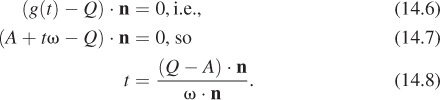
As an example, consider a surface defined by the plane through point Q with normal n. A suitable test function is
For every point P in the plane, f(P) = 0. For points on the side containing Q + n, f(P) > 0; for points on the other side, f(P) < 0.
An explicit equation or parametric equation defines a generator function for points in the plane in terms of scalar parameters. We can use such a function to synthesize points on the surface. The explicit form for a plane is
where h and k are two vectors in the plane that are linearly independent. For any particular pair of numbers u and v, the point g(u, v) lies on the plane. Chapter 7 gives both implicit and parametric descriptions for spheres and ellipsoids, and parametric descriptions of several other common shapes like cylinders, cones, and toruses. These, and more general implicit surfaces, are discussed in Chapter 24.
14.5.2.1. Ray-Tracing Implicit Surfaces
Implicit surface models are useful for ray casting and other intersection-based operations. For ray tracing, we take the parametric form of the ray with origin A and direction ω,
and solve for the point at which it intersects the plane by substituting into the plane’s implicit form and finding the roots of the resultant expression. We want to find a value t for which f(g(t)) = 0. That means
We can follow the same process for any surface whose equation admits an efficient closed-form solution after substituting the ray’s parametric form.
For a sphere of radius r about the point Q, we can use the implicit form f(P) = ||Q – P||2 – r2. Substituting the parametric form for the ray, and setting to zero, we get
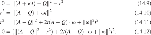
This is a quadratic equation in t, at2 + bt + c = 0, where a = ||ω||2, b = (A – Q) · ω, and c = ||(A – Q||2 – r2. It can be solved with the quadratic formula to find all intersections of the ray with the sphere.
(a) Write out the solutions using the quadratic formula, and simplify.
(b) What does it mean if one of the roots of the quadratic equation is at a value t < 0? What about t = 0?
(c) In general, if b2 – 4ac = 0 in a quadratic equation, there’s only a single root. What does this correspond to geometrically in the ray-sphere intersection problem?
More general quadratics can be used to determine intersections with ellipsoids or hyperboloids, while higher-order polynomials arise in determining the intersection of a ray with a torus, for example, and for more general shapes, the equation we must solve can be very complicated. Multiple roots of the equation that results from substituting the parametric line form into the function defining the implicit surface indicate multiple potential intersections. See Chapter 15 for further discussion of ray casting and interpreting its results.
What about implicit surfaces that do not admit efficient closed-form solutions? If the implicit surface function is continuous and maps points inside the object to negative values and points outside the object to positive values, then any root-finding method such as Newton-Raphson [Pre95] will find zero points, that is, it will find the surface. The term “implicit surface” usually refers to this kind of model and intersection algorithm.
Implicit surfaces that are defined by the sum of some simple basis functions with different origins are favored for modeling organic, “blobby” shapes (see Figure 14.16). This is called blobby modeling and metaball modeling [Bli82a].
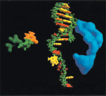
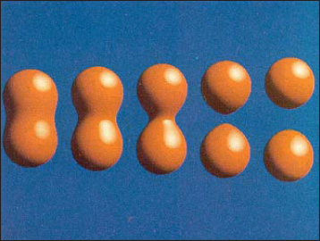
Figure 14.16: Blobby models, each defined by the isocontour of a sum of 3D Gaussian density functions [Bli82a]. (Credit: Courtesy of James Blinn © 1982 ACM, Inc. Reprinted by permission.)
14.5.3. Spline Patches and Subdivision Surfaces
We’ve seen that smooth shapes can be modeled by arbitrary expressions defining their surface curves through three dimensions and by the implicit surface defined by a parametric sum of fixed functions. Spline curves and patches and subdivision curves and surfaces are alternative representations that fall between these extremes. A spline is simply a piecewise-polynomial curve, typically represented on each interval as a linear combination of four predefined basis functions, where the coefficients are points. Thus, the curve can be represented by just storing the coefficients, which is very compact. A spline patch is a surface constructed analogously: a linear combination of several basis functions (each a function of two variables), where the coefficients are again points. This fixed mathematical form allows compact storage. The fact that the basis functions are carefully constructed, low-degree polynomials makes computations like ray-path intersection, sampling, and determining tangent and normal vectors efficient and fast. By gluing together multiple patches, we can model arbitrarily complex surfaces. (Indeed, spline patches are at the core of most CAD modeling packages.) There are many kinds of splines, each determined by a choice of the so-called basis polynomials. Graphics commonly uses third-order polynomial patches, which let us model surfaces with continuously varying normal vectors and no sharp corners. More general spline types, such as Nonuniform Rational B-Splines (NURBS), have historically been very popular modeling primitives. Splines may be rendered either by discretizing them to polygons by sampling, or by directly intersecting the spline surface, often using a root-finding method such as Newton-Raphson.
Subdivision surfaces are smooth shapes defined by recursive subdivision (using carefully designed rules) and smoothing of an initial mesh cage (see Figure 14.17). Because many modeling tools and many algorithms operate on meshes, subdivision surfaces are a practical method for adapting those tools to curved surfaces. They are especially convenient for polygon-based rendering because the mesh need only be subdivided down to the screen-space sampling density at each location. They have been favored for implementation in graphics hardware over other smooth surface representations because of this. For example, so-called tessellation, hull, and geometry shaders each map meshes to meshes inside the graphics hardware pipeline using subdivision schemes. As with all curve and surface representations, a major challenge is mixing sharp creases and other boundary conditions with smooth interiors. Representations that admit this efficiently and conveniently are an active area of research. At the time of this writing, that research has advanced sufficiently that the techniques are now being used in real-time rendering [CC98, HDD+94, VPBM01, BS05, LS08, KMDZ09].
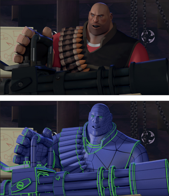
Figure 14.17: Top: A video-game character from Team Fortress 2 rendered in real time using Approximate Catmull Clark subdivision surfaces. Bottom: The edges of the subdivision cage (projected onto the limit surface) in black, with special crease edges highlighted in bright green. (Credit: top: © Valve, all rights reserved, bottom: Courtesy of Denis Kovacs; © 2010 ACM, Inc. Reprinted by permission.)
14.5.4. Heightfields
A heightfield is a surface defined by some function of the form z = f(x, y); it necessarily has the property that there is a single “height” z at each (x, y) position. This is a natural representation for large surfaces that are globally roughly planar, but have significant local detail, such as terrain and ocean waves (see Figure 14.18). The single-height property of course means that these models cannot represent overhangs, land bridges, caves, or breaking waves. By the Wise Modeling principle, you should only use heightfields when you’re certain that these things are not important to you. At a smaller scale, heightfields can be wrapped around meshes or other surface representations to represent displacements from the surface. For example, we can model a tile floor as a plane with a heightfield representing the grout lines. Heightfields used in this manner are often called displacement maps or bump maps [Bli78]. “Height” is of course relative to our orientation—it simply denotes distance from the base plane or surface along its normal, so we can use a heightmap to represent the wall of a log cabin simply by rotating our reference frame.
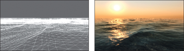
Figure 14.18: Left: The water surface heightfield in CryEngine2. Right: Real-time rendering of the dynamic heightfield [Mit07]. (Credit: Courtesy of Tiago Sousa, ©Crytek)
The height function can be implemented by a continuous representation, such as a sum of cosine waves, or by the interpolation of control points. The latter representation is particularly good for simulation, modeling, and measured data. The control points may be irregularly spaced so as to efficiently discretize the desired shape (e.g., a Triangulated Irregular Network (TIN), or the ROAM algorithm [DWS+97]), or they can be placed regularly to simplify the algorithms that operate on them. Because of their inability to model overhangs, heightfields are often used as a modeling primitive and then converted to generic meshes. Those meshes may be further edited without the heightfield constraint.
14.5.5. Point Sets
Heightfields, splines, implicit surfaces, and other representations based on control points all define ways to interpolate data from a fixed set of points to define a surface. As we increase the point density, the choice of interpolation scheme has less impact on the shape because the interpolation distances shrink. A natural approach to modeling complex arbitrary shapes is therefore to store dense point sets and use the most efficient interpolation scheme available. This is a particularly good approach for measured shapes, where the dense point sets naturally arise from the measurement process.
Point-based modeling often stores points at densities so high that the expected viewpoint and resolution will yield about one point per pixel, as shown in Figure 14.19. The interpolation thus need only cover gaps on the order of a pixel. Splatting is an efficient interpolation scheme under these conditions: Each point is rasterized as a small sphere (or disk facing the viewer) so that the space between points is covered but the overall shape conforms tightly to the point set. This is simply a form of convolution, and it is also equivalent to an implicit surface defined by a radial function that rapidly falls to zero (and is therefore trivial to evaluate). One can thus also directly ray-trace a point set, using the associated implicit surface.
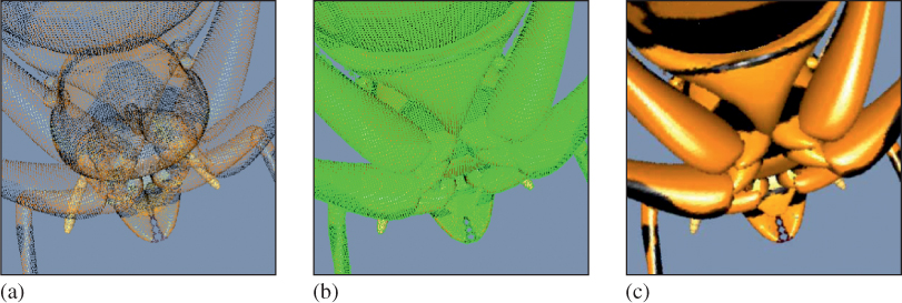
Figure 14.19: (a) A point set, with attached surface properties. (b) The gaps between points when rendered at this resolution. (c) The surface defined by splatting interpolation of the original points [PZvBG00]. (Credit: courtesy of Hanspeter Pfister, An Wang Professor of Computer Science, © 2000 ACM, Inc. Reprinted by permission.)
Because they are a natural fit for measured data but present some efficiency challenges for animation, modeling, and storage, point representations are currently more popular in scientific and medical communities than entertainment and engineering ones.
14.6. Distant Objects
Objects that have a small screen-space footprint or that are sufficiently distant that parallax effects are negligible present an opportunity to improve rendering performance. Under perspective projection, most of the viewable frustum is “far” from the viewer, and small-scale detail is necessarily less visible there. By simplifying the representation of distant or small objects, we can improve rendering performance with minimal impact on image quality. In fact, a simplified representation may even improve image quality because excluding small details prevents them from aliasing, especially under animation (see Section 25.4 for a further discussion of this).
14.6.1. Level of Detail
It is common to create geometric representations of a single object with varying detail and select among them based on the screen-space footprint of the object. This is called a level of detail (LOD) scheme [HG97, Lue01]. Discrete LOD schemes contain distinct models. To conceal the transitions, they may blend rendered images of the lower- and higher-detail models when switching levels, or attempt to morph the geometry. Continuous LOD schemes parameterize the model in such a way that these morphing transitions are continuous and inherent in the structure of the model.
To minimize the loss of perceived detail as actual geometric detail is reduced, structure that is removed from geometry is often approximated in texture maps. For example, the highest-detail variation of a model may contain only geometry, whereas a mid-resolution variation approximates some of the geometry in a normal or displacement map, and the lowest-resolution version alters the shading algorithm to approximate the impact of the implicit subpixel geometry.
Heightfields are a special case that offers a simple LOD strategy. Because the heightfield data is effectively a 2D elevation “image,” image filtering operations normally applied to rescaling (Chapter 19) can be applied to compute lower-resolution versions of the heightfield.
14.6.2. Billboards and Impostors
While the location within the viewport of a large, distant, static object changes with the camera’s orientation, the projection of that object is largely unchanged under small translations or rotations. Thus, a complex three-dimensional shape in the distance can be approximated by a flat, so-called billboard that bears a picture of the object rendered from approximately the current viewpoint. Such billboards are inexpensive to render because they are simply quadrilaterals with images mapped over them. Billboards may be used as the lowest level of detail in an LOD scheme, or as the only level of detail if it is known that the viewer will never approach the object. In some cases, billboards are also used for objects that are naturally flat, exhibit rotational symmetry, or for which orientation errors are difficult to notice. For example, a cluster of many leaves on a tree may be modeled as a single billboard, and likewise for a clump of many blades of grass. It is common to automatically rotate billboards toward the viewer during rendering to conceal their flat nature, although this is not appropriate in all cases. For example, distant tree billboards should rotate around their vertical axis to face the viewer, but should not rotate to face a viewer flying above the forest because doing so would make it appear that the trees had fallen over.
To increase realism, billboards can be augmented with surface normals or displacement maps [Sch97] that allow dynamic relighting.
Décoret et al. [DDSD03] proposed billboard clouds to automate for any model a process often employed by artists for foliage. The billboard cloud represents a single object with a collection of billboards oriented to incrementally minimize visual error in the rendered object (see Figure 14.20).
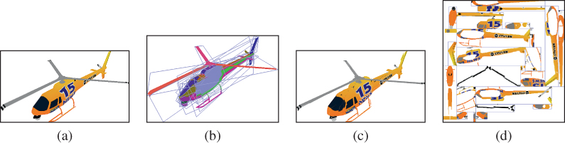
Figure 14.20: Example of a billboard cloud: (a) original model (5138 polygons), (b) false-color rendering using one color per billboard to show the faces that were grouped on each billboard, (c) view of the (automatically generated) 32 textured billboards, and (d) the billboards side-by-side. [DDSD03]. (Credit: Courtesy of Xavier Décoret, © 2003 ACM, Inc. Reprinted by permission.)
A limitation of individual billboards is that they cannot represent dynamic objects or views of objects as the observer approaches and parallax becomes nonnegligible. To address parallax, one could precompute many billboards, as was common in early 3D games such as Doom and Wing Commander, or develop warping strategies [POC05]. For dynamic billboards of specific objects, one could rig animation controls within the billboard itself [DHOO05, YD08]. However, a general solution is to simply rerender the billboards at runtime whenever the approximation error grows too large. These dynamic billboards are known as imposters [MS95], and they have seen widespread application for a variety of models, from terrain [CSKK99] to characters to clouds [HL01].
14.6.3. Skyboxes
It is often convenient to model parts of a scene as effectively “infinitely” distant. These may be rendered using finite distance for projection, but those distances are held constant regardless of the viewer’s translation. A frequent application is the sky, including clouds. For a character on the ground, the distance to objects in the sky is effectively constant and large, so there is no parallax or change in perspective with viewpoint movement. This is the ideal case for a billboard, except that planar geometry is inappropriate for wrapping around the horizon. A skybox or sky sphere is a geometric proxy for all distant objects. It wraps around the scene and translates so that the viewer is always at the center. The geometry for this proxy is arbitrary, so long as it surrounds the viewer. For example, it could be an icosahedron, tetrahedron, ...or teapot, and the shape will be indistinguishable from a sphere once the interior is painted with an appropriately projected image of the (virtual) distant scene geometry that it simulates. The choice of proxy geometry is therefore driven by the convenience and efficiency of generating that image under the given projection. Cubes and spheres both lend themselves to natural projections, and are therefore the most common models.
The term “skybox” is also used occasionally to refer to objects at finite distances such as building façades that provide a small amount of parallax but are in areas of the scene that the viewer will never enter. This is common, for example, in video games, where the player character’s movement is often constrained by natural obstacles but the designer wishes to efficiently represent a larger world than the navigable portion of the scene.
14.7. Volumetric Models
Most of the descriptions of matter that we’ve surveyed are surface representations. These are extremely efficient because they are mostly “empty”; they need not explicitly represent the space inside objects.
Volumetric modeling methods represent solid shapes rather than surfaces. Doing so enables richer simulation, both for dynamics and for illumination in the presence of translucency.
14.7.1. Finite Element Models
Finite element models are general divisions of solid objects into polyhedral chunks. These are very popular for detailed engineering simulation to model the internal forces within objects, heat and pressure propagation, and fluid flow. They are less popular for pure-rendering applications because they offer few advantages in that context over surface meshes.
A regular finite element subdivision into tetrahedrons or cubes offers additional advantages for modeling and simulation applications. Regularizing shapes allows constant-time random spatial access and stabilizes propagation. The tetrahedral division is good for simulation because the tetrahedron is the three-dimensional simplex—it is the simplest polyhedron, and is therefore a good primitive to model effects like fracture. The cube division naturally lends itself to a regular grid, making for straightforward representations, and is also easy to build hierarchies from. This representation is known as a voxel model. It is very common for fluid flow simulation and medical or geoscientific imaging, where the underlying source data are often captured on a regular grid.
14.7.2. Voxels
Voxels have gone in and out of favor for rendering, especially in entertainment. Figure 14.21 shows a contemporary game, Minecraft, which models the world with large voxels to intentionally inspire a building-block aesthetic. The game takes advantage of the efficiency of local graphlike operations on voxels to model all illumination and physical dynamics as cellular finite automata. Because the voxel representation requires only storage of the type of material in each cell (the position is implicit in the 3D array), the game is able to efficiently represent huge worlds with a single byte per cubic meter of storage—and large homogeneous regions are amenable to further compression. In comparison, modeling the same world even as a triangle list of cubes would require 12 triangles × 3 vertices/triangle × 3 floats/vertex × 4 bytes/float = 432 bytes per cubic meter, and would be less amenable to compression.
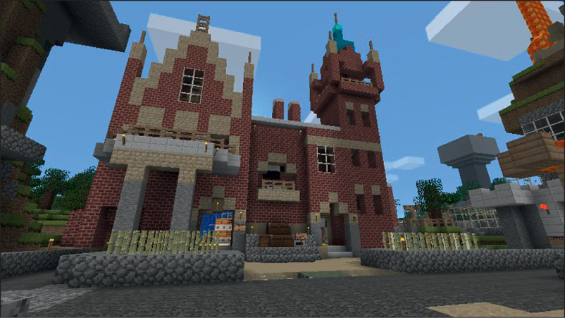
Figure 14.21: The game Minecraft models the entire world with 1 m3 voxels, enabling efficient, real-time illumination, simulation, and rendering for fully dynamic Earth-scale worlds.
Note that the scene in Figure 14.21 appears to have detail at finer resolution than the 1m3-voxel grid. For example, fences and reeds are represented by thin objects within a single grid cell. This is because that rendering system uses the voxels for simulation, but for rendering it replaces each with a proxy object that may be more detailed than a simple cube. This is an extreme form of geometry instancing. Geometry instancing is often used in less rigid scene representations to efficiently represent many similar elements. For example, a forest can be modeled with only a handful of individual tree models and a large number of tree locations and reference frames. One tree in the forest model then only requires storage for a pointer to a tree model and a coordinate frame, rather than for a unique tree geometry. Voxel scenes with relatively large-scale voxels can use a similar scheme to present higher apparent resolution than the voxel grid without the cost of modeling explicit fine-scale geometry for every voxel.
Figure 14.22 demonstrates a more refined use of voxels for efficient rendering of a high-resolution, static scene. Ray tracing through voxel grids is extremely efficient because the ray-surface intersections are trivial and the grid provides good spatial locality in the memory system. A tree data structure allows efficient encoding of large empty regions. Note that even when viewed up close, the voxels do not appear blocky. This image was rendered with a technique by Laine and Karras [LK10] that stores a surface plane along with shading information at each voxel, allowing surface reconstruction at apparently higher resolution along planes other than the grid itself. Several such techniques exist; one commonly used for fluid simulation is marching cubes [LC87] (and marching tetrahedrons [CP98]), which, given only density information stored in voxels, reconstructs some simple geometry in each voxel to produce a relatively smooth mesh (see Section 24.6).
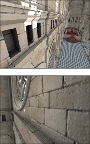
Figure 14.22: Voxel data created by high-resolution surface displacement, with local shadowing precomputed and stored in the voxel grid. The resolution is approximately 5 mm throughout the entire building, including outer walls that are not visible from the inside. The total size of the data in GPU memory is 2.7 GB. Laine and Karras’s ray caster was able to cast about 61 million rays per second when rendering this scene; in other words, to render 1M pixels at 60 fps by ray tracing in 2010 [LK10]. (Credit: Courtesy of Samuli Laine and Tero Karras, © 2010 ACM, Inc. Reprinted by permission.)
14.7.3. Particle Systems
Liquid or gaseous objects such as smoke, clouds, fire, and water are often modeled as particle systems [Ree83]. A particle system contains a set of individual particles, each of which can be efficiently simulated as a single point mass. There may be a large number of particles—say, thousands or millions—that play a role similar to individual molecules of gas or liquid. However, the simulation typically contains orders of magnitude fewer particles than a real-world scene would contain molecules. During rendering, the relatively low particle count is concealed by rendering a small billboard for each particle. This is similar to the splatting operation in point-based rendering. One usually calls a dynamic object with translucent billboards a particle system and a rigid object with opaque splats a point set. Section 14.10 describes methods for simulating translucency for both meshes and particles.
The billboard nature of particle systems can be revealed when the billboards intersect other geometry in the scene. Soft particles [Lor07] are a technique for concealing this intersection (see Figure 14.23). Soft particles become more translucent as they approach other geometry. Proximity is determined by reading a depth buffer during shading. The effect is particularly convincing for billboards that have high density and little visible structure, such as smoke.
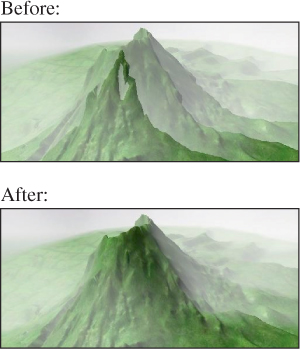
Figure 14.23: Top: The flat, discrete nature of this cloud particle system’s rendering billboards is revealed where it intersects the terrain mesh. Bottom: Adjusting the pixel shader to use the “soft particle” technique that fades out the billboard’s contribution with proximity to scene geometry conceals this artifact. (Credit: Courtesy of Tristan Lorach, NVIDIA)
14.7.4. Fog
Particles and voxels are discrete representations of amorphous volumetric shapes. Homogeneous, translucent volumes are amenable to continuous analytic representation. The classic application is atmospheric perspective, the relatively small-scale scattering of light by the atmosphere that desaturates distant objects in landscapes. A more extreme variation of the same principle is dense fog, which may be homogeneous over all space or vary in density with elevation.
True atmospheric perspective necessarily involves exponential absorption with distance, but it is often artistically desirable to present arbitrary control over the absorption rate. Homogeneous fog is implemented either during shading by blending the computed shade of each pixel toward the fog color based on distance from the viewer (e.g., in a pixel shader or employing the fixed-function glFog command in OpenGL), or by a 2D image post-process that performs the equivalent blending based on depth buffer values. An example of this blending to compute final color c′ from distance d, original color c, fog color f, and fog density parameter κ is (following the glFogf documentation)
The same approach can be applied to the scattering/attenuation of light when the camera is underwater. Much more sophisticated models of atmospheric scattering have been developed (e.g., [NMN87, Wat90, NN94, NDN96, DYN02, HP03]); this common exponential approximation is only the beginning.
Localized fog volumes (see Figure 14.24) can follow the same attenuation schemes as global ones, but the distance on which they are parameterized must measure only the extent traveled through the fog along the view ray, not the total distance from the observed surface to the viewer. This distance is computed by ray intersection with the bounding volume of the fog. Doing so within the shading algorithm for each pixel is reasonable provided that the bounding volume is geometrically simple. Half-plane, rectangular slab, and sphere volumes are common.
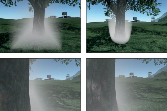
Figure 14.24: Box and ellipsoid fog volumes rendered by intersecting the view ray with an analytic volume inside a pixel shader. (Credit: Courtesy of Carsten Wenzel, © Crytek)
14.8. Scene Graphs
It is rare for large graphics systems to treat a scene as a single object. Instead, the scene is typically decomposed into a set of individual objects. This allows different model representations for different parts of a scene. It also reduces the memory size of objects that must be processed to both better accommodate computational limitations and provide manageable data sizes for the comprehension of human modelers and programmers. That is, this decomposition simply follows classic computer science and software engineering abstraction principles.
The data structure for maintaining the collection of objects in a scene is called a scene graph, where “graph” refers to pointers that express relationships between objects; you’ve already encountered a basic scene graph in the modeling hierarchy of Chapter 6, and the discussions of its traversal in Chapters 10 and 11. There are many scene-graph data structures. Deep trees are well suited to modeling and user-interface elements, where lots of fine-grained abstractions and a low branching factor match human design instincts. Relatively broad and shallow trees are often well suited to rendering on hardware with many parallel processing units and efficient object-level culling. Physical simulation often requires full graphs to express cyclic relationships in the simulation.
More-or-less aligned with the three goals of modeling and interaction, rendering, and simulation, there are three broad strategies for dividing the scene into elements. Classic scene graphs and shading trees divide a scene into semantic elements. For example, a character model might contain a “hair” node that is a child of a “head” node to enable easy coloring or replacement of hair. One might also attach a “skin color” property to a root node at the character’s torso that propagates that color property throughout the model. Semantic nodes are very similar to the cascading property schemes employed by text markup languages like HTML. This is not surprising; markup effectively describes a scene graph for text layout and rendering. Semantic scene graphics are nearly always directed acyclic graphs. A child node typically inherits shading and simulation properties from its parent in addition to a coordinate reference frame.
Physics scene graphs typically express constraint relationships (edges) between objects (nodes). These constraints are often joints. For example, a character’s wrist is a constraint that defines the coordinate transformation between the forearm and the hand. The constraints may be ephemeral; for example, a bouncing ball temporarily is constrained to not penetrate the ground (and perhaps experience limited lateral slip) on contact. Most dynamics systems include both prerigged character and machine articulation graphs and context-dependent constraint graphs for forces and contacts. See Chapter 35 for a discussion of dynamics and articulation data structures and algorithms.
Spatial data structures/scene graphs are the close analogue of general computer science data structures such as lists, trees, and arrays. They divide the scene into grids or trees that allow efficient spatial queries, such as “Which objects are within 4 m of my avatar?” Child nodes are typically contained within the bounding volumes of their parents. Spatial data structures are employed extensively in simulation and rendering. They are usually computed automatically. Efficient algorithms for building these data structures per-frame have recently emerged and this is an active area of research. Chapters 36 and 37 discuss modeling and interaction data structures and algorithms.
14.9. Material Models
As we said earlier, we conventionally think of objects as defined by their surfaces, which are the boundaries between them and other objects or the surrounding medium. But the solid nature of objects also has an effect on their interaction with light. Fortunately, we can limit our consideration to the interface between two media through which light propagates differently. That there are two media involved is essential. The appearance of a surface depends on both, although we commonly observe most objects in air, so this is not always apparent. For the moment, let us assume that objects are rendered in air so that we can define appearance using a single material parameter. We will return to the two-material case in Section 14.10.
The interaction of light and matter is quite simple. To a first approximation, each photon that strikes the surface has one of three fates: It is absorbed and converted into heat, it passes through the surface into the medium, or it reflects. The probability of each of these outcomes and the direction that scattered photons take after the interaction is governed by the materials involved and the microscopic angle of the plane of the surface near the location hit. A few simple laws from physics can describe the entire model.
However, we use high-level models that intentionally introduce more complexity than is present in these simple laws. Doing so lets us work with large numbers of photons in the aggregate and large (or at least, macroscopic) patches of surface. So, in exchange for complicating the material model, we can use simpler geometric surface models and light-sampling strategies. A more complex material model also allows aesthetic controls instead of physical ones, enabling artists to achieve their visions using intuition instead of measurement.
It is common practice to distinguish at least the following five artistically and perceptually significant phenomena.
1. Sharp specular (mirror) reflections, as seen on glass.
2. Glossy highlights and reflections, like the highlights on a waxed apple.
3. Shallow subsurface scattering, which produces matte Lambertian shading that is independent of the viewer’s orientation, such as observed with “flat” wall paint.
4. Deep subsurface scattering where light diffuses beneath the surface. This is what makes skin and marble appear soft.
5. Transmission, where light passes through a mostly translucent material such as water or fog, perhaps being slightly diffused along the way and refracted when it enters this medium.
Since these all just describe scattering (and lack of scattering, due to absorption), they are typically described by a scattering function. There are several variations, among them the bidirectional scattering distribution function (BSDF) for surface scattering, the reflectance-only variant (BRDF) for purely opaque surfaces, the BTDF for purely transmissive surfaces, and the BSSDF for describing both surface and shallow subsurface effects. BSDFs alone require fairly in-depth discussion of a specific rendering algorithm and surface physics to describe properly. Fortunately, one can also get by with a fairly simple model and application of it. A substantial portion of the pixels rendered in the past 30 years all used variations on the same simplified model, and it will likely be with us for some time.
In the following subsections we sketch the basic idea of a BSDF interface and one of the simple phenomenologically based models in common use today for opaque surfaces. We then return to some common approximations of transmission using compositing instead of BSDFs.
14.9.1. Scattering Functions (BSDFs)
Scattering can be described by a function (P, ωi, ωo) ![]() fs(P, ωi, ωo) that represents the probability density of light propagating in direction –ωi scattering to direction ωo when it strikes the surface at point P (see Figure 14.25). In general, a “brighter” or more reflective diffuse surface will have higher values of fs(). (The precise definition of fs is given in Chapter 26.)
fs(P, ωi, ωo) that represents the probability density of light propagating in direction –ωi scattering to direction ωo when it strikes the surface at point P (see Figure 14.25). In general, a “brighter” or more reflective diffuse surface will have higher values of fs(). (The precise definition of fs is given in Chapter 26.)

Figure 14.25: The vector ωi points toward the light source (represented by the star), so light propagates in direction –ωi. The light scatters at P and leaves in various directions ωo. The value fs(P, ωi, ωo) measures the scattering.
The use of fs is a mathematical convenience. In our programs, fs is typically defined in terms of some “basic” scattering function f defined by how it scatters light from a surface in the xz-plane whose outward normal vector is in the positive-y direction. As an example, a surface that preferentially scatters light in the normal direction could be modeled by
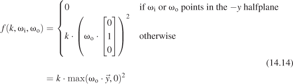
where k is a number between 0 and 1 describing how reflective the surface is (for this simple case, it reflects all wavelengths equally well). The function f is large when ωo is near the y-direction and small when it’s near the xz-plane. When we want to use f to represent the scattering from a surface that’s not oriented with its normal vector in the positive-y direction, we write fs so that it first transforms ωi and ωo into a new coordinate frame in which the surface normal at P is the second basis vector, and then apply f to these transformed vectors. Similarly, we might want to use f to represent a surface that’s “blotchy”—it’s more reflective in some places than others. We can do so by varying the value k as we move across the surface. The code for fs then has the structure shown in Listing 14.5.
Listing 14.5: Evaluating fs via a basic function f .
1 fs(P, wi, wo)
2 k = getReflectivity(P)
3 b1,b2,b3 = getBasis(P)
4 wiLocal = wi written in the b basis
5 woLocal = wo written in the b basis
6 return f(k, wiLocal, woLocal)
Most objects have varying appearance over their surface, like our blotchy sphere does. That is to say, fs varies over the surface of objects, not only because of the orientation of the surface, but because of varying surface properties. But the variation usually happens in the form just described: Some tool like texture mapping is used to determine the variation in the parameters that we want to pass to the basic scattering function f.
It would be awkward to work with a program in which there was actually a single BSDF for the entire scene that took a scene point as an argument and chose parameters based on it. For modularity, we want to have different BSDFs and attach them to surfaces freely. That is, “BSDF” should be a programmatic interface (i.e., type), and specific BSDFs such as those for glass and wood can be implementations of that interface. The spatial variation within a single logical material still presents a problem. That variation is typically parameterized in the surface’s own reference frame since the variation should transform with the object, appearing “painted on” the surface rather than projected through space onto it.
Two natural choices present themselves. One choice is to represent the BSDF for a single, small patch that is itself homogeneous. This pushes the problem of finding the local parameter variation back into the part of the program that sampled the surface location; for example, the ray-casting engine. In this case, we have fs(wi, wo) as the BSDF evaluation function.
The other choice is to represent the BSDF for an entire material with spatial variation and explicitly specify the point to be sampled in the material’s own space; for example, using texture coordinates. In this case, we have fs(u, v, wi, wo) as the BSDF evaluation function (although perhaps, since it’s a different function, we should use a name other than fs for it).
Neither choice is obviously superior; which to use depends on the constraints and design of the surface-sampling machinery. A similar choice can be made for the space in which to express the direction vectors. Thus far, we’ve followed the mathematical convention of assuming that ωi and ωo are in world space. However, the BSDF model is usually derived in the surface’s tangent space. Expressing the arguments in world space thus forces the BSDF to transform the arguments into the tangent space. That transformation may be explicit, or it may be implicit by developing all terms as dot products with the tangent and normal vectors. This also forces our “BSDF” representation to be aware of the local orientation of the surface—to be instantiated anew every time a point is sampled from the scene.
In this chapter, we choose to represent a sample of a surface rather than a BSDF. This means that a surface element encodes a position, reference frame, and any spatially varying parameters of the BSDF, as well as the BSDF itself. We favor this representation because it allows separating the ray-surface sampling and scattering portions of a renderer. That separation has pedagogical benefits because it allows us to consider the pieces of a renderer separately. It also has design benefits because the pieces become modular and we can mix different surface and scattering sampling methods. We do not consider the efficiency implications of this decision here, but note that it is used in several rendering libraries, such as PBRT (http://pbrt.org) and The G3D Innovation Engine (http://g3d.sf.net).
In practice, there are two different operations that fs must support. The first is direct evaluation: Given two directions, we wish to evaluate the function. This is used for direct illumination, where we have already chosen a light-transport path and wish to know the magnitude of the transport along it. The second is sampling. In this case, we are given either the incoming or the outgoing light direction and wish to choose the other direction with probability density proportional to fs, possibly weighted by projected area along one of the vectors.
For both direct evaluation and sampling, scattering such as by a mirror or lens that does not diffuse light and reflects or transmits a perfect image must be handled separately. The function fs “takes on infinite values” at the directions corresponding to reflection or transmission, which we call impulses. So we divide most operations into separate methods for the finite and impulse aspects.
![]() The API Principle
The API Principle
Design APIs from the perspective of the programmer who will use them, not of the programmer who will implement them or the mathematical notation used in their derivation. For example, a single BSDF f(ωi, ωo) mapped to a function API Color3 bsdf(Vector3 wi, Vector3 wo) is easy to implement but hard to use in a real renderer.
Listing 14.6 gives an interface for evaluating the finite part of f. This method abstracts the algorithm typically employed for direct illumination in a pixel shader or ray tracer. It is relatively straightforward to implement.
Listing 14.6: An interface for a scattering function’s direct evaluation (similar to G3D::Surfel).
1 class BSDF {
2 protected:
3 CFrame cframe; // coordinate frame in which BSDF is expressed
4
5 ...
6
7 public:
8
9 class Impulse {
10 public:
11 Vector3 direction;
12 Color3 magnitude;
13 };
14
15 typedef std::vector<Impulse> ImpulseArray;
16
17 virtual ∼BSDF() {}
18
19 /** Evaluates the finite portion of f(wi, wo) at a surface
20 whose normal is n. */
21 virtual Color3 evaluateFiniteScatteringDensity
22 (const Vector3& wi,
23 const Vector3& wo) const = 0;
24
25 ...
Listing 14.7 is an interface for the remaining methods needed for algorithms like photon mapping, recursive (Whitted) ray tracing, and path tracing. These are the methods for which the implementation and underlying mathematics are somewhat more complicated. We will not discuss them further here, except to note that the scattering methods are still straightforward to implement, given both the finite scattering density and the impulses, if we are willing to use rather inefficient implementations. There is nothing sacred about the particular methods we’ve included in this interface. In some implementations of path tracing, for instance, we want to sample with respect to a distribution proportional to the BSDF, without the extra weighting factor of ωi · n, and we might include a method for that in our interface.
Listing 14.7: An interface for a scattering function’s scattering and impulse methods.
1 class BSDF {
2 ...
3
4 /** Given wi, returns all wo directions that yield impulses in
5 f(wi, wo). Overwrites the impulseArray. */
6 virtual void getOutgoingImpulses
7 (const Vector3& wi,
8 ImpulseArray& impulseArray) const = 0;
9
10
11 /** Given wi, samples wo from the normalized PDF of
12 wo -> g(wi, wo) * |wi . n|,
13 where the shape of g is ideally close to that of f. */
14 virtual Vector3 scatterOut
15 (const Vector3& wi,
16 Color3& weight) const = 0;
17
18
19 /** Given wi, returns the probability of scattering
20 (vs. absorption). By default, this is computed by sampling
21 since analytic forms do not exist for many scattering models. */
22 virtual Color3 probabilityOfScatteringOut(
23 const Vector3& wi) const;
24
25 /** Given wo, returns all impulses for wi. */
26 virtual void getIncomingImpulses
27 (const Vector3& wo,
28 ImpulseArray& impulseArray) const = 0;
29
30
31 /** Given wo, samples wi from the normalized PDF of wi -> g(wi, wo) * |wi . n|. */
32 virtual Vector3 scatterIn
33 (const Vector3& wo,
34 Color3& weight) const = 0;
35
36
37 /** Given wo, returns the a priori probability of scattering (vs. absorption) */
38 virtual Color3 probabilityOfScatteringIn(const Vector3& wo) const = 0;
39
40 };
There are two sources for BSDF implementations. Measured BSDFs are constructed from thousands or millions of controlled measurements of a real surface. Measurement is expensive (or tricky to perform oneself), but it provides great physical realism. The data describing the BSDF is typically large but generally smooth, and thus amenable to compression.
Analytic BSDFs describe the surface appearance in terms of physically or aesthetically meaningful parameters. They are usually expressed as sums and products of simple functions that are zero for most arguments and rise in a smooth lobe over a narrow region of the parameter space. Those analytic BSDFs that model the underlying physics can be used predictively. We now describe some simple yet popular analytic BSDFs.
14.9.2. Lambertian
Lambert observed that most flat, rough surfaces reflect light energy proportional to the cosine of the angle between their surface normal and the direction of the incoming light. This is known as Lambert’s Law. It follows from geometry for surfaces with a constant BSDF because the projected area of the surface is proportional to the cosine of the incoming-light angle. A constant BSDF is named Lambertian because it follows this law.
Although few surfaces exhibit truly Lambertian reflectance, most insulators can be recognizably approximated by a Lambertian BSDF. The residual error is then addressed by adding other terms, as described in the following subsection.
Examples of nearly Lambertian surfaces are a wall painted with flat (i.e., matte) paint, dry dirt, and skin and cloth observed from several meters away. The primary error in approximating these as Lambertian is that they tend to appear shinier than predicted by a constant BSDF when observed at a glancing angle.
In practice, the approximately Lambertian appearance usually arises because the surface is somewhat permeable to light at a very shallow level and all directionality is lost by the time light emerges. Glossy highlights are caused by light preferentially reflecting close to the mirror-reflection direction. When that does not happen, the surface appears matte.
Listing 14.8 implements a Lambertian BSDF’s evaluate method. We specify a single “Lambertian constant” kL for each frequency band, that is, a Color3. The components of kL must each be in the range [0, 1]. They represent the reflectivity of the surface to each “color” of light. Larger values are brighter, so (1, 0, 0) appears bright red and (0.2, 0.4, 0.0) is a dark brown. Of course, few real surfaces truly have perfect absorption or perfect reflectance along any color channel. Many physically based rendering systems also tend to risk dividing by zero if any color channel is at either limit, so it is a good idea to select constants on the open interval (0, 1) in practice.
Listing 14.8: The finite direct evaluation portion of a simple Lambertian BSDF for surfaces such as walls covered in matte paint.
1 class LambertianBSDF : public BSDF {
2 private:
3 // Each element on [0, 1]
4 Color3 k_L;
5
6 public:
7 virtual Color3 evaluateFiniteScatteringDensity
8 (const Vector3& wi,
9 const Vector3& wo) const {
10 if ((wi.dot(cframe.rotation.getColumn(1)) > 0) &&
11 (wo.dot(cframe.rotation.getColumn(1)) > 0)) {
12 return k_L / PI;
13 }
14 else {
15 return Color3::zero();
16 }
17 }
18 ...
19 };
Note that there is no projected area factor in fs(P, ωi, ωo) = kL/π. That geometric factor must be accounted for by the renderer, as shown in Listing 14.11. We divide kL by π because the integral of the BSDF times the cosine of the angle of incidence must be less than one over the entire hemisphere above a planar surface to ensure energy conservation, and ![]() .
.
Because Lambertian appearance arises from well-diffused light, Lambertian reflectance is also called diffuse or perfectly diffuse reflection. We use the term “diffuse” to describe all nonspecular behavior.
14.9.3. Normalized Blinn-Phong
Phong introduced the phenomenological shading model [Pho75] described in Chapter 6. His model describes a surface that exhibits Lambertian reflection with a glossy highlight of adjustable sharpness.
The original Phong model has been reformulated as a BSDF and then extended by many practitioners. The currently preferred form remains phenomenologically based but has some basic properties that are desirable in a scattering model; for example, it conserves energy and obeys the projected area property. For a richer explanation of scattering models see Chapter 27. We simply present the model here in a form suitable for implementation.
This is the modern formalization, in terms of physical units, of the model that was described in Chapter 6. The replacement of Cd and Cs with kL and kg is appropriate for three reasons. First, “Lambertian” is a more specific name for the shape of the “diffuse” distribution; anything that isn’t an impulse is “diffuse,” but Phong prescribes a specific and geometrically well-founded Lambertian distribution for that term. Second, we’ve defined “specular” as a technical term for a mirror impulse, following its English definition and physics terminology, reserving “glossy” to denote reflection that’s somewhat or very concentrated in a particular direction. Third, this formulation is different from the original in both parameters and form. These k parameters are no longer potentially ambiguous RGB triples (each 0 ... 1), but constants representing the net probability over all directions of that term contributing to scattering.
The specific variant in Listing 14.9 includes the adjusted highlight term introduced by Blinn, the (implicit) projected area factor demanded by physics, and an approximate normalization factor introduced by Sloan and Hoffman [AMHH08] for energy conservation. Figure 14.26 shows the impact of varying the two glossy parameters of glossy coefficient and smoothness.
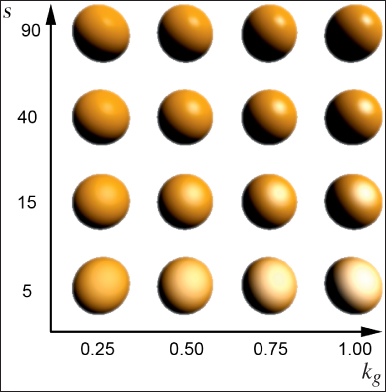
Figure 14.26: Sphere rendered with a single light source, using a Phong BSDF with a white kg and orange kL. kg increases to the right and s increases upward. (Credit: From Creating Games: mechanics, content, and technology by McGuire, Morgan and Jenkins, Odest Chadwicke © 2009. Reproduced with permission of Taylor & Francis Group LLC Books in the formats other book and textbook via Copyright Clearance Center)
Listing 14.9: Normalized Blinn-Phong BSDF without Fresnel coefficients, based on the implementation from Real-Time Rendering [AMHH08].
1 class PhongBSDF {
2 private:
3 // For energy conservation, ensure that k_L + k_g < 1 on each color channel
4 Color3 k_L;
5 Color3 k_g;
6
7 // “Smoothness” parameter; the exponent on the half-vector dot
8 // product.
9 float s;
10
11 public:
12
13 virtual Color3 evaluateFiniteScatteringDensity
14 (const Vector3& wi,
15 const Vector3& wo) const {
16
17 if ((wi.dot(cframe.rotation.getColumn(1)) <= 0) &&
18 (wo.dot(cframe.rotation.getColumn(1)) <= 0)) {
19 return Color3::zero();
20 }
21 const Vector3& w_h = (w_i + w_o).direction();
22 return k_L / PI + k_g * (8 + s) / (8 * PI) * pow(max(0.0, n.dot(w_h)), s);
23 }
24
25 ...
26 };
The Phong BSDF has three parameters. The Lambertian constant kL controls the color and intensity of matte reflection. The analogous kg controls the color and intensity of glossy reflection, which includes highlights produced by glossy reflection of bright light sources. A perfectly smooth reflective surface has a mirrorlike appearance. Rougher surfaces diffuse the mirror image, which produces the glossy appearance. The term including kg produces a teardrop-shaped lobe near the mirror-reflection direction when fs is graphed, so kg is often referred to as the magnitude of the glossy (or specular) lobe.
The smoothness parameter s describes how smooth the surface is, on an arbitrary scale. Low numbers, like s = 60, produce fairly broad highlights. This is a good model for surfaces like leather, finished wood, and dull plastics. High numbers, like s = 2000, produce sharper reflections. This is a better model for car paint, glazed ceramics, and metals.
The scale of s is not perceptually linear. For example, s = 120 does not produce highlights that have half the extent of s = 60 ones. It is therefore a good idea to expose a perceptual “shininess” parameter σ ![]() [0, 1] to artists and map it to s with a function such as s = 8192(1–σ).
[0, 1] to artists and map it to s with a function such as s = 8192(1–σ).
Most insulators exhibit colorless highlights, so kg is typically chosen to either be constant across color channels or have a hue opposite kL in order to sum to a gray or white appearance. Metals tend to have nearly zero Lambertian reflectance and a kg that matches the perceived color of the metal; examples include gold, copper, silver, and brass.
The normalization factor (8 + s)/(8π) increases the intensity of highlights as they grow sharper. This makes s and kG somewhat perceptually orthogonal and makes the energy conservation constraint simply kL + kg ≤ 1. The “8”s appear from rounding the constants in the true solution for the integral of the glossy term over the hemisphere to the nearest integer.
14.10. Translucency and Blending
We say that an object or medium is translucent when we can “see through it,” such as with glass, fog, or a window screen. For that to happen, some light from beyond the object must be able to pass through it to reach our eyes.
The phenomenon of translucency occurs when multiple scene locations directly contribute to the energy at a point in screen space. Under the ray optics modeled in this chapter, light rays do not interact with one another. For example, two flashlight beams pass through each other. Because they don’t interact, we can consider the energy contribution from each light ray independently. We then sum the contribution of all rays to a point. The property of light that describes this behavior (at least macroscopically) is called superposition. This property is what allows us to consider different wavelengths (colors) independently as well as describe light scattering for individual rays yet render all the light in a scene.
As with any other scene point, the incoming energy at a point on the image plane may arrive from multiple locations. The camera aperture blocks a majority of incoming directions, and in the limiting case of a pinhole camera, it blocks all but a single direction. In that case, a single ray exiting the virtual camera describes the path (albeit backward) along which light must have arrived. Yet in the presence of translucent surfaces, there may be multiple scene points along that eye ray that contribute because those points need not fully obscure the light coming from beyond them.
Given our model of surfaces, all light that passes through a surface to reach the camera is, by definition, indirect illumination. In other words, we can still render a single surface at each screen-space point. We just allow some light to scatter from behind the surface to in front of it. For a material like green glass, the scattering may “color” the outgoing light by transmitting some frequencies more than others.
Transmission of many kinds can naturally be represented by the BSDF models that we’ve already discussed. Yet those models are too computationally expensive for current real-time rendering systems. Just as was the case for scattering and surface models, it is common to intentionally introduce both approximations and a more complicated model for transmission to gain both expressive control and improved performance. The common approximation to translucency phenomena is to render individual surfaces in back-to-front order and then compose them by blending, a process in which the various colors are combined with weights. The blending functions are arbitrary operators that we seek to employ to create phenomena that resemble those arising from translucency. In general, this model forgoes diffusion and refraction effects in order to operate in parallel at each pixel, although it is certainly possible to include those effects via screen-space sampling (e.g., [Wym05]) or simply using a ray-tracing algorithm. Most graphics APIs include entry points for controlling the blending operation applied as each surface is rendered. For example, in OpenGL these functions are glBlendFunc and glBlendEquation. We give examples of applying these in specific contexts below.
There are multiple distinct causes for translucency. Distinguishing among them is important for both artistic control and physical accuracy of rendering (either of which may not be important in a particular application). Because all reduce to some kind of blending, there is a risk of conflating them in implementation. The human visual system is sensitive to the presence of translucency but not always to the cause of it, which means that this sort of error can go unnoticed for some time. However, it often leads to unsatisfying results in the long run because one loses independent control over different phenomena. Some symptoms of such errors are overbright pixels where objects overlap, strangely absent or miscolored shadows, and pixels with the wrong hue.
To help make clear how blending can correctly model various phenomena, in this section we give specific examples of applying a blending control similar to OpenGL’s glBlendFunc. The complete specification of OpenGL blending is beyond what is required here, changes with API version, and is tailored to the details of OpenGL and current GPU architecture. To separate the common concept from these specifics, we define a specific blending function that uses only a subset of the functionality.
If you are already familiar with OpenGL and “alpha,” then please read this section with extra care, since it may look deceptively familiar. We seek to tease apart distinct physical ideas that you may have previously seen combined by a single implementation. The following text extends a synopsis originally prepared by McGuire and Enderton [ME11].
14.10.1. Blending
Assume that a destination sample (e.g., one pixel of an accumulation-buffer image; see Chapter 36) is to be updated by the contribution of some new source sample. These samples may be chosen by rasterization, ray tracing, or any other sampling method, and they correspond to a specific single location in screen space.
Let both source and destination values be functions of frequency, represented by the color channel c. For each color channel c, let the new destination value ![]() be
be
where δ and σ are functions that compute the contributions of the old destination value d and the source value s. Let BlendFunc(senum, denum) select the implementation of the δ and σ functions. To enable optimization of common cases in the underlying renderer, APIs generally limit the choice of σ and δ to a small set of simple functions. Hence the arguments to BlendFunc are enumerated types rather than the functions themselves. For generality, let senum and denum have the same type.
A partial list of the blending function enumerants and the functions to which they correspond (which we’ll extend a bit later) is:
ONE: bc(s,d) = 1
ZERO: bc(s,d) = 0
SRC_COLOR: bc(s,d) = sc
DST_COLOR: bc(s,d) = dc
ONE_MINUS_SRC_COLOR: bc(s,d) = 1 – sc
ONE_MINUS_DST_COLOR: bc(s,d) = dc
To make the application of BlendFunc clear, we now examine two trivial cases in a common scene. There exist alternative and more efficient methods for achieving these specific cases in OpenGL than what we describe here, specifically the blending enable bit and write mask bits, but we describe the general solution to motivate blending functionality.
Consider a static scene containing a wall covered in red latex paint, a pinhole camera, and a thin, flat blue plastic star that is suspended between the wall and the camera, occupying about half of the image in projection. Let these objects be in a vacuum so that we need not consider the impact of a potentially participating medium such as air. Now consider a sample location near the center of the star’s projection.
Blue plastic is reflective, so light incident on the star at the corresponding point within the scene is either absorbed or reflected. Assume that we have somehow computed the incident light and the reflective scattering. Let s describe the radiance reflected toward the screen-space sample location. If we are in the midst of rendering, then the image that we are computing may already have some existing value d at this location, either the value with which it was initialized (say, dc = 0 W/(sr m2)) or perhaps some “red” value if the wall was rendered into the image first.
Any light transported from the background wall along the ray through our sample and the camera’s pinhole must necessarily be blocked by the blue star. So we don’t care what the preexisting value in d is. We simply want to overwrite it. For this case, we select BlendFunc(ONE, ZERO), yielding the net result
This is not very exciting, and it seems like a silly way of specifying that the new value overwrites the existing one. It makes a little more sense in the context of a hardware implementation of the blending function. In that case, there is some arithmetic unit tasked with updating the frame buffer with the new value. The unit must always be semantically configured to perform some function, however trivial.
Say that we’re rendering the scene by rasterization. Rasterization is just a way of iterating over screen-space sample locations. We typically choose to iterate over the samples arising from the projection of object boundaries (i.e., surfaces). However, one can also choose to rasterize geometry that does not correspond to an object boundary as a way of touching arbitrary samples. For example, deferred shading typically rasterizes a bounding volume around a light source as a conservative method for identifying scene locations that may receive significant direct illumination from the source. If rasterizing some such volume that lies entirely within the vacuum, how do we blend the resultant contribution? One method is BlendFunc(ZERO, ONE), yielding the net result
which allows the preexisting value in the image to remain. Here, the rasterized surface is perfectly transparent, meaning that it is truly invisible to light. Why bother rasterizing when we’ll just discard the source color? One answer is that there are more attributes than just radiance stored at a pixel. One might want to mark an area of the depth or stencil buffer without affecting the image itself. This occurs, for example, when implementing stenciled shadow volumes by rasterization. Another answer is that we may want to change the blending weights per-sample to selectively discard some of them, as discussed in Section 14.10.2.
14.10.2. Partial Coverage (α)
Let us return to the scene containing a thin blue star floating in front of a red wall, introduced in Section 14.10.1. One way to model the blue star is with a single two-sided rectangle and a function defined on the rectangle (say, implemented as a texture map) that is 1 at locations inside the star and 0 outside the star. This function, whose value at a sample is often denoted α, describes how the star covers the background.
The coverage in this case is associated with the sample of the source object that is being rendered, so we should denote it αs. An implementation likely contains a class for representing radiance samples at three visible frequencies (red, green, and blue) and a coverage value as
1 class Color4 {
2 float r;
3 float g;
4 float b;
5 float a;
6 };
To leverage the concept of coverage as a way of masking transparent parts of the rectangle, we introduce two new blending enumerants:
SRC_ALPHA: bc(s,d) = sa
ONE_MINUS_SRC_ALPHA: bc(s,d) = 1-sa
The blending mode BlendFunc(SRC_ALPHA, ONE_MINUS_SRC_ALPHA) yields
which is linear interpolation by sα. Our coverage value at each point is either 0 or 1, as befits the physical model of the star: At every point sample the rectangle enclosing the star is either completely opaque and blocks all light from the background, or completely transparent and allows the background to be seen.
Rendering under such a binary coverage scheme with a single sample per pixel will generate aliasing, where the edges of the star appear as stair steps in the image. If we increase the number of samples per pixel, we will obtain a better estimate of the fraction of the star that covers an individual pixel. For example, in Figure 14.27, the outlined pixel is about 50% covered by the star and 50% covered by the background. However, the estimate would be poor if we used three samples instead of four, and even the four samples from the diagram can produce an error of ±12.5% coverage for pixels with less even coverage. Taking many samples per pixel is of course an expensive way to evaluate partial coverage by analytically defined shapes.
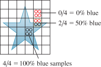
Figure 14.27: An ideal blue vector star shape rasterized on a low-resolution pixel grid. The boxes of the grid are pixels. The circles represent samples at which we are computing coverage.
We’ve seen this problem before, with texture maps encoding reflectance. The MIP-mapping solution developed in Chapter 20 works for coverage as well as reflectance. Imagine a prefiltered coverage map for the star rectangle in which the outlined pixel in Figure 14.27 is a single texel (one pixel in a texture-map image). Its coverage value is the integral of binary coverage over that texel, which is sα = 0.3. This integral is called partial coverage. Equation 14.20 holds for partial coverage as well as binary coverage; in this case it is called the over operator because it represents the image of a partially covering s lying over the background d.
Order matters, however. The over operator assumes that we’re rendering surfaces in back to front order (the Painter’s Algorithm described in Section 36.4.1) so that we always composite nearer objects over farther ones.
Note that sα encodes the fraction of coverage, but not the locations of that coverage within the texel. One interpretation of sα is that it is the probability that a sample chosen uniformly at random within the texel will hit the opaque part of the rectangle instead of the transparent part. For the star, the probability remains at the extremes of 0 and 1 except at texels along the edge. For other shapes, nearly every texel encodes some kind of edge. Consider a screen door, for example. We might paint a texture that has sα as 1 and 0 in alternating rows and columns at the highest resolution. Such a texture has maximum spatial frequencies, so it could produce significant aliasing. However, after a single MIP level, the texture contains entirely fractional values.
An advantage of the probabilistic interpretation of partial coverage is that it allows us to describe the result of successive applications of blending for different surfaces without explicitly representing the high-frequency coverage mask in the result image d′. For example, we can render the back wall as viewed through two identical screen doors by computing the final destination color ![]() for each channel c
for each channel c ![]() r, g, b as
r, g, b as
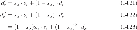
The pitfall of this interpretation is that it assumes statistical independence between the subpixel coverage locations for each s-layer. If the two doors are perfectly aligned (assume a parallel projection to make this easy), then this assumption does not hold because the second door provides no new occlusion of the background. In this case, the second door is precisely behind the first and is invisible to the camera. Therefore, we should have obtained the result ![]() , and not the one from Equation 14.23.
, and not the one from Equation 14.23.
Equation 14.23 contains the result we expect on average; that is, if the locations covered by the doors are statistically independent. This is generally what one wants, but if there is some underlying reason that the coverage should be correlated between surfaces, then Equation 14.23 will give incorrect results. For example, when the sα value results from thin-line rasterization, many thin lines may naturally align in screen space (say, the support cables on a suspension bridge) and yield an incorrect result.
The classic paper by Porter and Duff [PD84] that canonicalized blending carefully analyzes all coverage cases and is specific about the statistical independence issue. Yet it is very easy to implement incorrectly. For example, the OpenGL 3.0 and DirectX 10 APIs contain an alpha-to-coverage feature that converts sα back to a binary visibility mask when placing multiple samples within a pixel. That feature yields incorrect compositing results, as it is specified, because the mask contains a fixed pattern based on the sα value. Thus, the subpixel locations covered by two surfaces with equal, fractional α are always perfectly correlated in those APIs. This tends to give undesirable results for overlapping translucent surfaces. Enderton et al. [ESSL11] describe the problem and one solution: Choose the coverage based on a hash of the depth value and screen-space position.
We’ve discussed the coverage of the surface, but what about the coverage of ![]() , the result image? Consider a case where we are rendering an image of the contribution of all surfaces between a depth of 1 m and 2 m from the camera. We would then like to composite this over another image containing the result for objects at 2 m and farther. In that case, some pixels in our close image may be completely transparent, and others may have partial or complete coverage. If we again assume statistical independence of subpixel locations covered by different surfaces, we can composite coverage itself by
, the result image? Consider a case where we are rendering an image of the contribution of all surfaces between a depth of 1 m and 2 m from the camera. We would then like to composite this over another image containing the result for objects at 2 m and farther. In that case, some pixels in our close image may be completely transparent, and others may have partial or complete coverage. If we again assume statistical independence of subpixel locations covered by different surfaces, we can composite coverage itself by
thus creating a composite value d that itself acts like a surface with partial coverage.
14.10.2.1. Premultiplied α
Note that in the preceding section, sc never appeared in isolation. Instead, it was always modulated by sα. Our interpretation of this was that s is a surface with α coverage of a screen-space area, and that the covered parts had color sc, or more formally, emitted and scattered radiance sc toward the viewer. The net contribution from s is thus scsα.
It is common practice to store colors with premultiplied alpha, in the form (srsα, sgsα, sbsα, sα). This has several advantages. For example, it saves a few multiplication operations during compositing and resolves the ambiguity in the meaning of sc for a surface with sα = 0. The latter point becomes significant in the (underdetermined) image processing problem of matting, where an algorithm tries to recover scsα, sα, and dc from the composite ![]() .
.
14.10.3. Transmission
Partial coverage was a model that allowed us to describe fine but macroscopic structures like lace or a window screen using simple geometric shapes and a statistical measure of coverage. In that case, the covered parts of the surface were completely opaque and the uncovered parts transmitted all light because they were filled by the surrounding medium, such as air.
If we ignore refraction (the phenomenon of light bending when it enters a new medium), we can extend partial coverage to microscopic structures. Consider an extremely thin pane of colorless glass. An incident light ray will either strike a glass molecule on the surface and reflect or be absorbed, or pass through the empty space between molecules (this model is physically simplistic, but phenomenologically viable). We can let α represent the coverage of space by glass molecules and render the glass using the partial coverage model. This is in fact done frequently, although adding a bit more sophistication to our model allows us to remove the extremely thin and colorless models to better describe a range of transmissive media.
Green glass appears green because it transmits green light. If you hold a piece of green glass over a black background, then it appears mostly black because it reflects little green light. If we continue with the microscopic partial coverage model, then sg ≈ 0 for the glass. The green glass in fact reflects little light at any frequency, so sr ≈ sg ≈ sb = 0. We can’t describe the appearance of green glass over a white surface using a single coverage value α, because the coverage must be large for red and blue light (so that they are blocked) and low for green light (so that it transmits). We need to extend our coverage representation. Let sc be the color of light reflected or emitted at the surface near frequency c, and 1 – tc be the microscopic coverage of frequency c by the surface, that is, t is the amount of light transmitted. We retain the sα value for representing macroscopic partial coverage by a transmissive medium. We can now express the composition of the surface over the background by holding out the background by 1 – t and then adding the contribution due to s.
To implement this in code, we use the SRC_COLOR enumerant to selectively block light from the background and then make a second pass to add the contribution from the surface:
1 // Selectively block light from the background
2 // where there is coverage
3 SetColor(t * s.a + (1 - s.a));
4 BlendFunc(ZERO, SRC_COLOR);
5 DrawSurface();
6
7 // Add in any contribution from the surface itself,
8 // held out by its own coverage.
9 SetColor(s);
10 BlendFunc(SRC_ALPHA, ONE);
Note that this example implements transmission by a thin surface that may itself have only partial macroscopic coverage. In the case where that coverage is complete and the surface itself scatters no light, the entire example reduces to simply:
1 SetColor(t);
2 BlendFunc(ZERO, SRC_COLOR);
3 DrawSurface();
We’ve presented this in a form similar to the OpenGL API for real-time rasterization rendering. The mathematics can be applied per-pixel in another rendering framework, such as a ray tracer. Doing so is common practice, although we suggest that if you’ve already written a ray tracer with well-structured ray-scattering code, then it may be trivial to implement much more accurate transmission with a BSDF than with blending. If you choose to employ the blending model, the code might look something like:
1 Radiance3 shade(Vector3 dirToEye, Point3 P, Color3 t, Color4 s, ...) {
2 Radiance3 d;
3 if (bsdf has transparency) {
4 // Continue the ray out the back of the surface
5 d = rayTrace(Ray(P - dirToEye * epsilon, -dirToEye));
6 }
7
8 Radiance3 c = directIllumination(P, dirToEye, s.rgb, ...);
9
10 // Perform the blending of this surface’s color and the background
11 return c * s.alpha + d * (t * s.alpha + 1 - s.alpha);
12 }
Our blending model for transmission at this point supports frequency-varying (colored) transmission and a distinct color scattered by or emitted at the surface. Yet it still assumes an infinitely thin object so that transmission can be computed once at the surface. For an object with nonzero thickness, light should continue to be absorbed within the material so that thicker objects transmit less light than thinner ones of the same material.
Consider the case of two thin objects held together, assuming sα = 1 macroscopic coverage and 1–trgb microscopic coverage, that is, transmission. We expect the first object to transmit t of the light from the background: d′ = td; and the second to transmit t of that, for a d″ = t2d net contribution from the background, as in our previous double-compositing example of macroscopic partial coverage. Now consider the case of three such thin objects; the net light transmitted will be t3d. Following this pattern, a thick object composed of n thin objects will transmit tnd. The absorption of light is thus exponential in distance, as we suggested in Equation 14.13.
We can still apply the simple compositing model if we precompute an effective net transmission coefficient t for the thick object based on the distance x that light will travel in the medium, that is, its cross section along the ray. Three common methods for computing this thickness are tracing a ray (even within the context of a rasterization algorithm), rendering multiple depth buffers so that the front and back surfaces of the object are both known (e.g., [BCL+07]), or simply assuming a constant thickness. It is common to express the rate of absorption by a constant k. The net transmission by the thick object along the ray is thus t = e–kx. The thin-blending model can then be applied with this constant. This exponential falloff is a fairly accurate model and k can be computed from first principles; however, given the rest of the rendering structure that we’ve assumed in this section, it is more likely to be chosen aesthetically in practice.
14.10.4. Emission
It is often desirable to render objects that appear to glow without actually illuminating other surfaces. For example, car tail lights and the LEDs on computer equipment likely contribute negligible illumination to the rest of the scene but themselves need to appear bright in an image. These effects may be simulated by rendering the scene normally and then additively blending the emissive component as if it were a new surface rendered using BlendFunc(ONE, ONE).
Some particularly attractive effects are due to such emission by a medium that is itself seemingly transparent. Examples include the light from a neon bulb, lightning, science fiction “force fields,” and fantasy magical effects. That the underlying surface is invisible in these cases is irrelevant—the additive blending of the emissive component is unchanged.
14.10.5. Bloom and Lens Flare
Lens flare and bloom are effects that occur within the optical path of a real camera. One could model the real optical path, but to merely achieve the phenomena it is much more effective to additively blend contributions due to additional geometry over the rendered frame using BlendFunc(ONE, ONE). Bloom simulates the diffusion of incident light within lenses and the saturation of the sensor. It is typically simulated by blurring only the brightest locations on-screen and adding their contribution back into the frame. Lens flare arises from multiple reflections between lenses within the objective. It is typically simulated by rendering a sequence of iris (e.g., hexagonal or disk) -shaped polygons along a 2D line through bright locations, such as the sun, on-screen.
14.11. Luminaire Models
A computer graphics luminaire is a source of light. The luminaires we encounter in daily life vary radically in the spectra of light that they emit, their surface areas, and their intensities. For example, the sun is large and distant, a spotlight is bright and small, and a traffic light is relatively dim and colored. The luminaires we might encounter in a virtual world expand this variation further; for example, a cave of phosphorescent fungus, a magic unicorn’s aura, or the navigation lights on a starship.
Before we can present luminaire models, we must first discuss light. You know that light is energy (in photons) that propagates along rays through space and scatters at surfaces. There are many models of light in computer graphics, but they all begin by representing the rate at which energy is passing through a point in space. We give a brief synopsis here and defer extensive coverage until Chapter 26. One can render images from the models in this chapter without understanding the motivation and physics behind light transport. However, we recommend that after rendering your first images you read Chapter 26 to build a deeper understanding.
14.11.1. The Radiance Function
Consider a point X in space at which we wish to know the illumination. This is frequently on some surface in the scene, but it need not be. The amount of light incident at X from direction ω is denoted L(X, ω). This implicitly defines a function L of two variables, X and ω, which is called the radiance function, also known as the plenoptic function. To be clear, the argument ω denotes the direction of propagation. If there’s a photon passing through the point P, traveling in direction ω, then L(P, ω) ≠ 0, while it’s quite possible that L(P, –ω) = 0. By convention, we’ll restrict to the case where ω is a unit vector. The units of L are watts per square meter-steradian, W · m–2 · sr–1. Surface areas are measured in units of square meters, and steradians are the spherical analog of angular measure, called solid angle. An angle can measure a 1D region on a 2D unit circle in the plane, and you might express the rate of a quantity passing through that 1D region “per radian.” We measure the amount of energy passing through a 2D region (a solid angle) on a unit sphere in 3-space “per steradian.”
It is useful to know that radiance is conserved along a ray through empty space. Thus, if we know L(X, ω), then we also know L(X + tω, ω) for t > 0 so long as there is no occluding object within distance t of X along that ray.
14.11.2. Direct and Indirect Light
We distinguish the light that arrives at a point directly from a luminaire from light that arrived indirectly after reflecting off some surface in the scene. For example, near an outdoor swimming pool, sunlight shines directly on the top of your head, but it also reflects off the water to indirectly strike the bottom of your chin. If there were no indirect light, then the bottom of your chin would appear completely unilluminated. The indirect light arises from interaction between the luminaire and the scene, so we consider it part of the light transport model and not the luminaire model.
14.11.3. Practical and Artistic Considerations
Listing 14.10 gives a typical base class for a set of light-class implementations. Its methods support the practical aspects of incorporating light sources into a renderer, not the physical aspects of light emission.
Listing 14.10: A base class for all light sources, with trivial implementation details omitted.
1 /** Base class for light sources */
2 class Light {
3 public:
4 const std::string name() const;
5
6 virtual CoordinateFrame cframe() const;
7
8 /** for turning lights on and off */
9 virtual bool enabled() const;
10
11 /** true for physically-correct lights */
12 virtual bool createsLambertianReflection() const;
13
14 /** true for physically-correct lights */
15 virtual bool createsGlossyReflection() const;
16
17 /** true for physically-correct lights */
18 virtual bool createsGlobalIllumination() const;
19
20 /** true for physically-correct lights */
21 virtual bool castsShadows() const;
22
23 //////////////////////////////////////////
24 // Direct illumination support
25
26 /** Effective area of this emitter. May be finite,
27 zero, or infinite. */
28 virtual float surfaceArea() = 0;
29
30 /** Select a point uniformly at random on the surface
31 of the emitter in homogeneous coordinates. */
32 virtual Vector4 randomPoint() const = 0;
33
34 /** Biradiance (solid-angle-weighted radiance) at P due
35 to point Q on this light, in W / m^2. Q must be a value
36 previously returned by randomPoint(). */
37 virtual Biradiance3 biradiance
38 (const Vector4& Q, const Point3& P) const = 0;
39
40 //////////////////////////////////////////
41 // Photon emission support
42
43 /** Total power; may be infinite */
44 virtual Power3 totalPower() const = 0;
45
46 /** Returns the position Q, direction of propagation w_o, and
47 normalized spectrum of an emitted photon chosen with
48 probability density proportional to the emission density
49 function for this light. */
50 virtual Color3 emitPhoton(Point3& Q, Vector3& w_o) const = 0;
51 };
We assign a reference frame (cframe) to each light source. For a light at a finite location, this is the centroid of the emitter and a reference orientation. For infinitely distant sources (i.e., directional sources), this is a reference frame and a convenient location within the scene for displaying GUI affordances to manipulate the source.
14.11.3.1. Nonphysical Tools
It is often useful to manipulate the interaction of lights and the scene in nonphysical ways. These may depart from physics for artistic intent, but they may also be used to compensate for flaws in the rendering model itself. That is, the right model with the wrong data (or vice versa) can’t produce the correct image, so sometimes we have to compensate for known limitations and approximations by intentionally violating physics in order to make the net result appear more realistic. The class shown in Figure 14.10 contains several of these tools, in the form of light sources that don’t cast shadows, or don’t participate in the computation of Lambertian reflection, for instance. Of course, the renderers that use this class must honor such settings for them to have an effect.
Luminaires that do not create glossy reflection (e.g., highlights) provide so-called “fill” or “diffuse” light. These create perceptual cues of three-dimensional shape and softness, approximating global illumination and subsurface scattering. Glossy-only sources create explicit highlights but no other shading. These are useful to model the perceptual cues from practical lights. Practical lights are the light sources that appear to be in the scene, as opposed to the invisible ones that are actually lighting most of it. The term comes from film and theatre production; as an example, in a film set of a dining room, very little illumination actually comes from the candles on a table and the scene is more likely to receive illumination primarily from bright off-camera stage lights. Glossy-only sources are particularly useful for creating the perception of windows without dealing with the net impact of those windows on scene light levels. The “Lambertian” and “glossy” reflectance properties properly belong to the surface material, not the light, so using these properties assumes a specific material and shading model.
In the real world, the light from an emitter may experience an unbounded number of scattering events before it is perceived. It is often artistically useful to shine a light on a specific object without incurring the computational cost or global implications of multiple scattering events. A direct, local, or nonglobal light source only scatters light from the first surface it encounters toward the viewer. Beware that the term “local” is also used in lighting models to refer to lights that are at a finite distance from visible parts of the scene.
One may wish to selectively disable shadow casting by lights. This can save the computational cost of computing visibility as well as eliminate shadows that may be visually confusing, such as those cast outward from a carried torch.
14.11.3.2. Applying the Interface to Direct Illumination
The key methods for incorporating the Light class into a renderer are randomPoint and radiance. The randomPoint method selects a point on the surface of the emitter uniformly at random with respect to surface area. (The term “selected uniformly at random” is defined precisely in Chapter 30; for now, treat it as meaning “every point is equally likely to be chosen.”) Because the point may be infinitely distant from other parts of the scene, we represent the return value as a homogeneous vector. For lights that have varying intensity over their surface, a better choice of interface might be to select the emitter point with probability proportional to the amount of light emitted at that point. Even further elaborations might involve choosing luminaire points in a way that’s random but guarantees fairly even distribution of the points and avoids clustering. Stratified sampling, discussed briefly in Chapter 32, is one such method.
The radiance method returns the incident radiance at a scene point due to a point on the emitter (which was presumably discovered by calling randomPoint), assuming that there is no occluding surface between them. We separate generation of the emitter point from estimating the radiance from it so that shadowing algorithms can be applied. We must know the actual scene point and not just the direction to it in order to compute the radial falloff from noncollimated sources.
Listing 14.11 shows how to apply these methods to compute the radiance scattered toward the viewer due to direct illumination. In the listing, point P is the point to be shaded, w_o is the unit vector in the direction from P to the eye, n is the unit surface normal at P, and bsdf is a model of how the surface scatters light (see Chapter 27 for a full discussion of physically based scattering).
Listing 14.11: Direct illumination from an arbitrary set of lights.
1 /** Computes the outgoing radiance at P in direction w_o */
2 Radiance3 shadeDirect
3 (const Vector3& w_o, const Point3& P,
4 const Vector3& n, const BSDF& bsdf,
5 const std::vector<Light*>& lightArray) {
6
7 Radiance3 L_o(0.0f);
8
9 for (int i = 0; i < lightArray.size(); ++i) {
10 const Light* light = lightArray[i];
11
12 int N = numSamplesPerLight;
13
14 // Don’t over-sample point lights
15 if (light->surfaceArea() == 0) N = 1;
16
17 for (int s = 0; s < N; ++s) {
18 const Vector4& Q = light->randomPoint()
19 const Vector3& w_i = (Q.xyz() * P - P * Q.w).direction();
20
21 if (visible(P, Q)) { // shadow test
22 const Biradiance3& M_i = light->biradiance(Q, P);
23 const Color3& f = bsdf.evaluateFiniteScatteringDensity(w_i, w_o, n);
24
25 L_o += n.dot(w_i) * f * M_i / N;
26 }
27 }
28 }
29
30 return L_o;
31 }
If this is your first encounter with code like that shown in Listing 14.11, simply examine it for now and then treat it as a black box. A fuller explanation of the radiometry that leads to this implementation and motivates the abstractions appears in Chapter 32. A brief explanation of the derivation of this implementation appears in the following section.
14.11.3.3.  Relationship to the Rendering Equation
We now attempt to reconcile the “light” that’s used in the traditional graphics pipeline (e.g., in Chapter 6) with the physically based rendering model that is described in Chapter 31. The key idea is that if we measure light in units of biradiance,6 then classic graphics models can function as simplified versions of the physics of light and the rendering equation.
6. We are not aware of a preexisting name for solid-area weighted radiance measured at the receiver, so we introduce the term “biradiance” here to express the idea that it incorporates two points. This quantity is distinct from radiosity (which considers the whole hemisphere), irradiance (which is measured at the emitter’s surface), radiant emittance (likewise), and other quantities that commonly arise with the same units.
This material appears in this chapter because it constitutes a conventional approximation to the real physics of light, which we wanted to introduce before the full theory. It of course also serves readers encountering this section after reading Chapters 26 and 31, or with previous experience in graphics systems.
For a scene with only point lights and Phong BSDFs in which we have, numSamplesPerLight = 1, Listing 14.11 degenerates into the familiar OpenGL fixed-function shading algorithm. The framework presented in this chapter provides some explanation of what the lighting parameters in OpenGL “mean.” That puts us on a somewhat more solid footing when we attempt to render scenes designed for classic computer graphics point sources within a physically based renderer. It also leads us to the settings perhaps most likely to produce a realistic image under rendering APIs similar to OpenGL.
For all scenes, Listing 14.11 implements direct illumination in the style employed both for algorithms like path tracing and for explicit direct illumination under rasterization. It is an estimator for the terms in the rendering equation due to direct illumination (Figure 14.28 shows the key variables, for reference). The perhaps unexpected radiant emittance units arise from a change of variables from the form in which we often express the rendering equation. That is, we commonly express the scattered direct illumination as
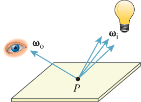
where the domain of integration is the hemisphere ![]() + above the point P at which we are computing the illumination.
+ above the point P at which we are computing the illumination.
That would lead us to an implementation like:
1 repeat N times:
2 dw_i = 2 * PI / N;
3 L_i = ...;
4 L_o += L_i * bsdf.evaluate(...) * n.dot(w_i) * dw_i;
However, path tracing and other algorithms that employ explicit direct illumination sampling tend to sample over the area of light sources, rather than over the directions about the shaded point.
We must change integration domains from ![]() + to the surfaces of the lights; that entails making the appropriate change of variables. Consider a single light with surface region ΔA and unit surface normal m at Q (see Figure 14.29).
+ to the surfaces of the lights; that entails making the appropriate change of variables. Consider a single light with surface region ΔA and unit surface normal m at Q (see Figure 14.29).
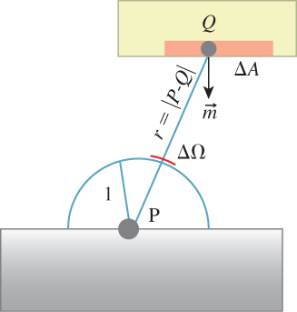
Figure 14.29: The small, solid-angle Δ![]() and a corresponding small region ΔA on the luminaire’s surface.
and a corresponding small region ΔA on the luminaire’s surface.
The distance from P to the surface region ΔA is approximately r = ||Q – P||, while the distance from P to Δ![]() is exactly 1. (Recall that Δ
is exactly 1. (Recall that Δ![]() is a small region on the unit sphere around P.) If the region ΔA near Q were not tilted (i.e., if m and ωi were opposites), then its area would be r2 times the area of Δ
is a small region on the unit sphere around P.) If the region ΔA near Q were not tilted (i.e., if m and ωi were opposites), then its area would be r2 times the area of Δ![]() . The tilting principle of Section 7.10.6 says that the area is multiplied by a cosine factor. So the area of ΔA is approximately r2|m · ωi| times the area of Δ
. The tilting principle of Section 7.10.6 says that the area is multiplied by a cosine factor. So the area of ΔA is approximately r2|m · ωi| times the area of Δ![]() , with the approximation getting better and better as the region Δ
, with the approximation getting better and better as the region Δ![]() shrinks in size. Thus the change of variable, as we go from dωi to dA (often denoted by some symbol like
shrinks in size. Thus the change of variable, as we go from dωi to dA (often denoted by some symbol like ![]() is
is ![]() . We can now rewrite Equation 14.25, substituting S(Q – P) for ωi,
. We can now rewrite Equation 14.25, substituting S(Q – P) for ωi,
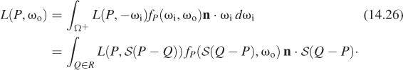
where we’ve used P – Q instead of Q – P in some places to avoid excess negative signs or absolute values.
One way to estimate the integral of any function g over any region is to pick a random point X in the region, evaluate g(X), and multiply by the area of the region. (We discuss this in far more detail in Chapter 30.) If we repeat this process, then each individual estimate will probably not be very good, but their average will get better and better the more (independent) points we choose. Applying this to the integral above, if we choose N points Qj ![]() R on the luminaire, we can estimate the reflected light as
R on the luminaire, we can estimate the reflected light as
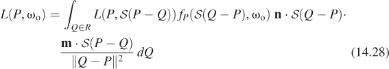
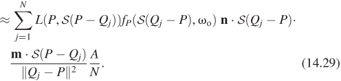
Another interpretation of the factor ![]() is that each sample Qi represents one Nth of the area of the luminaire.
is that each sample Qi represents one Nth of the area of the luminaire.
We can simplify the notation in this expression somewhat by letting ωi,j be the unit vector S(Qj – P) from P to the jth sample point Qj on the luminaire. We then have
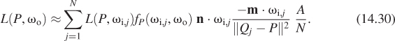
If we denote by M(P, Qj, m) the value
then the reflected radiance becomes
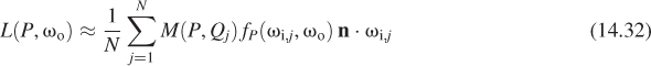
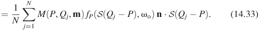
The units of M are m2 times the units of radiance times the units of dω/dA, which are steradians per meter squared; the net units are W/m2. We’ll call M the biradiance, to indicate its dependence on two points, one on the luminaire and one on the receiving surface. We caution that this is not a standard radiometric term.
We’ll return to the interpretation of M in a moment, but the structure of this equation leads us to pseudocode that follows the structure of Listing 14.11:
1 repeat N times:
2 // Computed by the emitter
3 L_i = ...
4 M_i = L_i * max(-m.dot(w_i), 0.0f) * A / ||P - Q||^2
5
6 // Computed by the integrator (i.e., renderer)
7 if there is an occluder on the line from P to Q then M_i = 0
8 L_o += M_i * bsdf.evaluate(...) * n.dot(w_i) / N
Thus, one interpretation of the deprecated fixed-function OpenGL Phong shading and (to some degree) shading in WPF is that the light “intensities” correspond to the function M, whose units are watts per square meter. This particular quantity is not one that has a standard name in radiometry, however, and we will not mention it again. It’s also worth noting that in most simple rendering using the classical model, the 1/r2 falloff is not actually modeled, so the claim that what’s used as an intensity is M is somewhat suspect. What’s true is that if you wish to use the classical model to approximate physical reality, then you should use the 1/r2 falloff, and you should assign luminaires “intensity” values computed according to the formula for M.
14.11.3.4. Applying the Interface to Photon Emission
Algorithms such as bidirectional ray tracing and photon mapping track the path of virtual photons forward from the light source into the scene. These virtual photons differ from the real photons that they model in two respects. The first distinction is that their state includes a position, a direction of propagation, and the power of the photon. Real photons transport energy, but rendering considers steady-state light transport, so it tracks the rate of energy delivery. It is more accurate to say that each virtual photon models a stream of photons, or that it models a segment of a light-transport path. The second distinction from real photons is that trillions of real photons contribute to a single real image, whereas renderers typically sample only a few million virtual photons (although each represents a stream of photons, so in truth many more real photons are implicitly modeled).
The first step of photon tracing is to emit photons from the sources in the scene. Listing 14.12 shows how to use our light interface to sample numPhotons-emitted virtual photons with a probability density function proportional to the power of each light source.
Listing 14.12: Generating numPhotons photons from a set of lights; for example, for photon mapping.
1 void emitPhotons
2 (const int numPhotons,
3 const Array<Light*>& lightArray,
4 Array<Photon>& photonArray) {
5
6 const Power3& totalPower;
7 for (int i = 0; i < lightArray.size(); ++i)
8 totalPower += lightArray[i]->power();
9
10 for (int p = 0; p < numPhotons; ++p) {
11 // Select Lwith probability L.power.sum()/totalPower.sum()
12 const Light* light = chooseLight(lightArray, totalPower);
13
14 Point3 Q;
15 Vector3 w_o;
16 const Color3& c = light->emitPhoton(Q, w_o);
17
18 photonArray.append(Photon(c*totalPower/numPhotons, Q, w_o));
19 }
20 }
14.11.4. Rectangular Area Light
We now model a planar rectangular patch that emits light from a single side, as shown in Figure 14.30. This will be a so-called “Lambertian emitter,” which means that if we restrict our field of view so that the emitter fills it entirely, then we perceive the emitter’s brightness as the same regardless of its orientation or distance. We describe the light source’s orientation by an orthonormal reference frame in which m is the unit normal to the side that emits photons and u and v are the axes along the edges. The edges have lengths given by extent and the source is centered on point C.
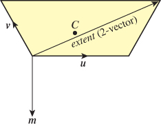
The total power emitted by the light is Phi. This means that if we increase extent, the illumination level in the scene will appear constant but the emitter’s surface will appear to become darker since the same power is distributed over a larger area.
The radiance (W/(m2 sr)) due to a point Q on a Lambertian emitter, emitted in any direction ω, is the total emitted power (W) divided by the area (m2) of the emitter and the so-called “projected solid angle” (sr)
For a discussion of this and other radiometric terms, see Section 26.7.1.
We can now compute the biradiance at P due to Q. Let ωi = S(Q – P). Light leaving Q in direction –ωi arrives at P traveling in direction –ωi. The leaving light has radiance Φ/(Aπ sr) by Equation 14.35. So
assuming that P is on the emitting side of the light source and there is an unoccluded line of sight to Q. Listing 14.13 gives an implementation of the key Light methods for such a light source based on this derivation.
Listing 14.13: A model of a single-sided rectangular Lambertian emitter.
1 class RectangularAreaLight : public Light {
2 private:
3 // Orthonormal reference frame of the light
4 Vector3 u, v, m;
5
6 Vector2 extent;
7
8 // Center of the source
9 Point3 C;
10
11 Power3 Phi;
12
13 public:
14
15 ...
16
17 Vector4 randomPoint() const {
18 return Vector4(C +
19 u * (random(-0.5f, 0.5f) * extent.x) +
20 v * (random(-0.5f, 0.5f) * extent.y), 1.0f);
21 }
22
23 float area() const {
24 return extent.x * extent.y;
25 }
26
27 Power3 power() const {
28 return Phi;
29 }
30
31 Biradiance3 biradiance(Vector4 Q, Vector3 P) const {
32 assert(Q.w == 1);
33 const Vector3& w_i = (Q.xyz() - P).direction();
34
35 return Phi * max(-m.dot(w_i), 0.0f) /
36 (PI * (P - Q.xyz()).squaredLength());
37 }
38 };
14.11.5. Hemisphere Area Light
A large hemispherical light source that emits inward is a common model of the sky or other distant parts of the environment. Listing 14.14 adapts the concepts from the rectangular area light source to such a dome. Two natural extensions to this model are to incorporate a coordinate frame so that the hemisphere can be arbitrarily centered and oriented, and to modulate the power over the dome by an image to better simulate complex environments and skies with high variability.
Listing 14.14: A model of an inward-facing hemispherical light dome, centered at the origin and with rotational symmetry about the y-axis.
1 class HemisphereAreaLight : public Light {
2 private:
3 // Radius
4 float r;
5 Power3 Phi;
6
7 public:
8
9 ...
10
11 Vector4 randomPoint() const {
12 returnVector4(hemiRandom(Vector3(0.0f, 1.0f, 0.0f))*r, 1.0f);
13 }
14
15 float area() const {
16 return 2 * PI * r * r;
17 }
18
19 Power3 power() const {
20 return Phi;
21 }
22
23 Biradiance3 biradiance(Vector4 Q, Vector3 P) const {
24 assert(Q.w == 1 && Q.xyz().length() == r);
25
26 const Vector3& m = -Q.xyz().direction();
27 const Vector3& w_i = (Q.xyz() - P).direction();
28
29 return Phi * max(-m.dot(w_i), 0.0f) /
30 (PI * (P - Q.xyz()).squaredLength());
31 }
32 };
14.11.6. Omni-Light
An omnidirectional point light (omni-light or [ambiguously] point light) is a luminaire that emits energy equally in all directions and is sufficiently small that it has negligible bounding radius compared to the distance between the source and nearby scene locations. A true point light would have to have a surface that was infinitely bright to produce measurable emission from zero surface area, and so could not exist. However, there are many luminaires whose volume is negligible compared to the scale of the scenes in which they are encountered, such as the bulb in a flashlight or the LED lights on the dashboard of a car. It is also common to approximate a larger light source with an omni-light at its center, and some surrounding proxy geometry that appears to the viewer to be the luminaire but does not actually emit light in the lighting simulation. For example, a campfire might be modeled by a flickering omni-light floating in the midst of the flames, which were themselves rendered by a particle system.
An omni-light is typically modeled by its total power emission in all directions, Φ. This is a scalar measured in watts; it can be represented as a 3-tuple to express power at the red-green-blue frequencies. Real-life experience provides good estimates for the power of omni-lights in our scene, since lightbulbs are labeled in watts of power consumed. As we said earlier, the emitted light from a 100 W bulb is about 4 W. A fluorescent bulb is about six times more efficient, so a bulb labeled “equivalent to a 100 W incandescent bulb” also emits about 4 W of visible light, but it consumes less electric power in doing so.
Let Q be the center of an omni-light. The radiance at P directly from the luminaire must arrive from direction ωi = S(Q – P). That is, ωi points to the light, from the surface. It is known as the light vector and is sometimes also denoted ![]() (although we avoid that notation because it is confusingly similar to the radiance function notation L(·)).
(although we avoid that notation because it is confusingly similar to the radiance function notation L(·)).
The omni-light is an abstraction of a very small spherical source. We can estimate the radiant emittance due to an omni-light by estimating the effect of ever-smaller spherical sources. The only way that the size of a source enters our formula is in the surface area term A in Equation 14.37. However, that term appears both in numerator and denominator, so it cancels and the end result is independent of the area. The cosine term also varies from point to point for an area source but is constant for the omni-light’s point source; one might say that this is another way that size “matters.” Regardless, the conclusion is that we can use exactly the same formula for the biradiance from area and point sources.
The biradiance at P due to the omni-light at Q (see Figure 14.31) is given by
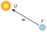
if there is no scene point on the open line segment from Q to P; it is 0 if there is an occlusion.
Note that we could say that the effective radiance is
that is, it is proportional to the total power of the luminaire and falls off with the square of distance from the luminaire. In fact, if we were to insert that expression into a renderer it would yield the desired image so long as ||Q – P|| was “sufficiently large.” However, this is not actually a true radiance expression because it is not conserved along a ray—it falls off with distance because our omni-light in fact has the physically impossible zero surface area, which leads it to create a physically impossible radiance field in space. Note that both the radiance and the biradiance approach infinity as ||Q – P|| ![]() 0. It is common practice to clamp the maximum biradiance from an omni-light, since when that distance is small our original assumption that the distance to the luminaire is much greater than the size of the luminaire is violated and the resultant estimated light intensity is greater than intended. A less efficient but more accurate correction would be to actually model the luminaire as an object with nonzero surface area (such as a sphere) when the distance is less than some threshold.
0. It is common practice to clamp the maximum biradiance from an omni-light, since when that distance is small our original assumption that the distance to the luminaire is much greater than the size of the luminaire is violated and the resultant estimated light intensity is greater than intended. A less efficient but more accurate correction would be to actually model the luminaire as an object with nonzero surface area (such as a sphere) when the distance is less than some threshold.
There is no illumination from the omni-light at locations that do not have an unobstructed line of sight. These regions form the shadows in an image. The boundary of the shadows from an omni-light will be “hard,” with a distinct curve across a surface that distinguishes lit from shadowed. This is unlike the area sources, which produce “soft” shadows with blurry silhouettes. A lighting algorithm such as shadow mapping that evaluates light visibility at lower precision than the radiance magnitude can appear to produce soft shadows from a point light. This is in fact an artifact of reconstruction from an aliased set of samples. Nonetheless, it may be visually pleasing in practice.
14.11.7. Directional Light
For an omnidirectional point light that is far from all locations in the scene, ωi and L(P, –ωi) due to the light vary little across the scene. A directional light is an omni-light with the further simplifying approximation that it is so far from the rest of the scene that ωi and L can be treated as constant throughout the scene. This eliminates some of the precision and modeling challenges of placing a point light very far away, while giving a reasonable model for a distant light source such as the sun.
We could model the total power of the distant point light, but it is typically enormous and “distant” is ambiguous, so it is easier to model the (constant) incident radiance at points in the scene by simply letting L(P, ω) = L0 for ωi directed exactly toward the light and 0 for all other directions. A useful constant to remember is that, for points on the surface of the Earth, L0 (in the visible spectrum) due to the sun is roughly 1.5 × 10⁶ W/m2sr. The total power of light in the visible spectrum arriving from all points of the sun at a region of the Earth’s surface is about 150 W/m2. Both of these, of course, vary with time of day, season, and latitude.
14.11.8. Spot Light
A spot light models an omni-light shielded by “barn door” flaps or a conical shade. Theatre lights, flashlights, car headlights, and actual spot lights are examples of real-world sources for which this model is appropriate (see Figure 14.32). It is common to choose to model the occluding portion as a perfectly absorptive sphere with a round iris through which light emerges. It is assumed to be perfectly absorptive so that we can neglect the complex reflections that occur on the silvered reflector of a headlight and flashlight. The iris is made round because that allows us to test whether a ray passes through it using a simple threshold of a dot product. A round iris produces a cone of light.


Figure 14.32: A theatre light with square “barn doors” (left), and a spot light with a round iris, matching our model. (Credit: top: Jim Barber/Shut-terstock, bottom: Matusciac Alexandru/Shutterstock)
Let Φ be the total power of the omni-light inside the blocker. It is convenient to specify this rather than the total power actually emitted. Doing so allows a lighting artist to adjust the spot-light cone independently of the observed brightness of objects within the cone.
Let 0 ≤ θ ≤ π be the measure of the angle between the axis and side of the emitted light cone. Note that θ = π is an iris fully opened so that there is no blocker and θ = 0 is completely closed. Beware of conventions here. Some APIs use radians, some use degrees. Also, some specify the full cone angle and some the half-angle as we have done here.
The measure of the solid angle subtended by a cone with angle measure 0 ≤ θ ≤ π between the axis and side is
The fraction of the emitter that is visible through the barn doors is therefore
so the externally observed power Φ′ of an omni-light of power Φ occluded by barn doors is
which is the Light::power value required for implementation in an importancesampling renderer.
Spot lights with θ ≤ π/4 are used extensively in rendering because they provide reasonable resolution for a planar projection of light space. That is, by placing a camera at the light, facing along its axis and with field of view matching the cone angle, one can render the light’s view of the scene with reasonably small distortion at the edges. This technique is used in shadow maps, for example, which are depth images from the light’s perspective, and reflective shadow maps, which are color images from the light’s perspective. Six spot lights, cropped down to square projections, can cover the six faces of a cube and represent shadowing from an omni-directional light.
Another application of light-space projection is a projective spot light. Real theatre lights are often modified by placing a gobo or cookie slide immediately outside the light source’s iris (see Figure 14.33). This colors or selectively blocks emitted light, projecting an image or shape onto the scene. In computer graphics, one can modulate the incident light at a point P in the scene by the value stored in an image at the corresponding location in the light’s projection of P to achieve this effect. This is used to create nonround and nonuniform spot-light apertures, to simulate the complex patterns of real spot-light reflectors, and to simulate shadows from off-screen objects, such as a spinning fan in a ventilation duct.
Figure 14.33: A photograph of spiral patterns created by real gobos in spotlights (Credit: R. Gino Santa Maria/Shutter-stock.com).
14.11.9. A Unified Point-Light Model
This section describes a model for luminaires with extents that are small in comparison to the distance between them and the points to be shaded. Under this definition of small, each luminaire can be approximated as a single point. This unifies several common light models. It was introduced and favored particularly for fixed-function graphics processors but remains widespread due to its simplicity.
A fixed-function unit implements a specific algorithm directly in circuitry or microcode. Such units are often controlled by parameters but cannot perform general-purpose computations the way that a programmable unit or general-purpose processor can. That is, they are not computationally equivalent to Turing machines. A processor typically contains a mixture of programmable and fixed-function units. For example, few architectures allow the programmer to alter the cache replacement strategy, but most allow arbitrary arithmetic expressions within programs. Graphics architectures may embed entire rendering algorithms in fixed-function logic. Fixed-function hardware naturally limits the programmer’s expression. However, it is extremely power-efficient and is less expensive to design and produce than general-purpose computation units. Thus, hardware architects face a design tradeoff based on current costs and goals.
At the time of this writing, fixed-function graphics units have gone in and out of fashion several times. Fixed-function lighting logic is currently eschewed in most devices, although at least one (the Nintendo 3DS [KO11]) released in 2011 embraces it.
We do not recommend the unified model presented in this section for new implementations built on programmable shading or software-based rendering APIs. The model is difficult to incorporate in a useful way into a physically based rendering system, limits the flexibility of the lighting model, and is a weaker abstraction than the models presented in subsequent chapters.
It remains important to be familiar with the model inspired by fixed-function logic for several reasons. Both legacy devices and a handful of new devices still use this model. The model may return to favor in the future. Many programmable graphics pipelines are still based around the fixed-function lighting model because they evolved from fixed-function implementations or must work with assets and tools originally designed for those implementations.
The basic idea of the model is that we can represent spot, directional, and omni-lights with a single, branchless lighting equation for a spot light with homogeneous parameters. The center of the spot light is (x, y, z, w), where w = 1 indicates a spot or omni-light and w = 0 indicates a directional light. If we parameterize the angle between the axis of the spot light and the edge of its cone, then an angle of π radians gives an omnidirectional light. The only remaining issue is radial falloff. In the real world, the total power observed at distance r from a uniform spherical emitter whose radius is much smaller than r is proportional to 1/r2. We can generalize this by computing a value M that involves an inverse quadratic:
If we define a and r by
then we can rewrite the formula for M as
This strange expression lets us represent a point emitter that experiences non-physical falloff to approximate a local area source or distant point source ...or simply to satisfy an artistic vision. In this context, a directional source can be parameterized by the attenuation constant ![]() = (1, 0, 0). This source will produce equal intensity at all points in the scene, and that intensity is comparable to what a local source with power Φ one meter from a surface would produce.
= (1, 0, 0). This source will produce equal intensity at all points in the scene, and that intensity is comparable to what a local source with power Φ one meter from a surface would produce.
The resulting interface (Listing 14.15) follows the spirit of the OpenGL fixed-function lighting model, albeit with slightly varying units and border cases. We do not recommend this model for physically based rendering.
Listing 14.15: A simple unified model for spot, directional, and omni light sources.
1 class PointLight : public Light {
2 private:
3
4 /** For local lights, this is the total power of the light source.
5 For directional lights, this is the power of an equivalent
6 local source 1^m from the surface. */
7 Power3 Phi;
8
9 Vector3 axis;
10
11 /** Center of the light in homogeneous coordinates. */
12 Vector4 C;
13
14 Vector3 aVec;
15
16 float spotHalfAngle;
17
18 ...
19 };
Listing 14.16: PointLight methods for direct illumination.
1 Vector4 PointLight::randomPoint() const {
2 return C;
3 }
4
5 Biradiance3 biradiance
6 (const Vector4& Q, const Point3& P) const {
7 assert(C == Q);
8
9 // Distance to the light, or zero
10 const float r = ((Q.xyz() - P) * Q.w).length();
11
12 // Powers of r
13 const Vector3 rVec(1.0f, r, r * r);
14
15 // Direction to the light
16 const Vector3& w_i = (Q.xyz() - P * Q.w).direction();
17
18 const bool inSpot = (w_i.dot(axis) >= cos(spotHalfAngle));
19
20 // Apply radial and angular attenuation and mask by the spotlight cone.
21 return Phi * float(inSpot) / (rVec.dot(aVec) * 4 * PI);
22 }
Listing 14.17: PointLight methods for photon emission.
1 Power3 PointLight::totalPower() const {
2 // the power actually emitted depends on the solid angle of the cone; it goes to
3 // infinity for a directional source
4 return Phi * (1 - cos(spotHalfAngle)) / (2 * C.w);
5 }
6
7 Color3 PointLight::emitPhoton(Point3& P, Vector3& w_o) {
8 // It doesn’t make sense to emit photons from a directional light with unbounded
9 // extent because it would have infinite power and emit practically all photons
10 // outside the scene.
11 assert(C.w == 1.0);
12
13 // Rejection sample the spotlight cone
14 do {
15 w_o = randomDirection();
16 } while (spotAxis.dot(w_o) < cos(spotHalfAngle));
17
18 P = Q.xyz();
19
20 // only the ratios of r:g:b matter
21 const Color3& spectrum = Phi / Phi.sum();
22 return spectrum;
23 }
14.12. Discussion
Each of the approximations and representations presented in this chapter has its place in graphics. Different constraints—on processor speed, bandwidth, data availability, etc.—create contexts in which they made (or make) sense. And while processors get faster, new constraints, like the limited power of mobile devices, may revive some approximations for a time. You should therefore regard these not only as currently or formerly useful tricks of the trade, but as things that are potentially useful in the future as well, and which provide examples of how to approximate things effectively within a limited resource budget.
14.13. Exercises
Exercise 14.1: Give an example of an arithmetic expression in which the commutativity does not hold for all operations; for example, in which evaluating left-to-right instead of following the usual order of operations gives an incorrect result.
Exercise 14.2: We said that direct mapping of the range [0, 2b – 1] to [–1, 1] precludes the exact representation of zero. Explain why. (You may find it easiest to start with the case b = 1.)
Exercise 14.3: Write a function that converts a triangle strip to a triangle list (a.k.a. triangle soup).
Exercise 14.4: Write a function that converts a triangle fan to a triangle strip. You may need to introduce degenerate triangles along edges.
Exercise 14.5: Consider a program that represents the world using a 3D array of opaque voxels; for simplicity, assume that they are either present or not present. Most rendering APIs use meshes, not voxels, so this program will have to convert the voxels to faces for rendering. Each filled voxel has six faces. But because the voxels are opaque, most of the faces in the scene do not need to be rendered—they are between adjacent filled voxels and can never be seen.
Give an algorithm for iterating through the scene and outputting only the faces that can be observed.
Exercise 14.6: Draw a computer science tree data structure representing the scene graph for an automobile, with the nodes labeled as to the parts that they represent.
Exercise 14.7: Consider a green beer bottle on a white table, in a night club lit with only red lights (assume each represents a narrow frequency range). What are the observed colors of the bottle, the table in the bottle’s shadow, and the table out of the bottle’s shadow?
Exercise 14.8: Implement disk and sphere Lambertian emitters in the style of Listing 14.13.
Exercise 14.9: Implement an arbitrary mesh Lambertian emitter in the style of Listing 14.13.