
Chapter 25. Meshes
25.1. Introduction
Back in Chapter 8, we introduced meshes as a way to represent shapes in computer graphics. We now return to examine meshes in more detail, because they dominate present-day graphics. The vertex-and-face-tables model we introduced in Chapter 8 is widely used to represent triangle meshes, which are almost universally used in hardware rendering, because triangles are automatically convex and planar and there’s only one possible way to linearly interpolate values at the three vertices of a triangle. Quad meshes, in which each face has four vertices, are also interesting in various situations. Indexing a regular planar quad mesh is very simple compared to indexing a regular planar triangle mesh, for instance. On the other hand, quads are not necessarily planar, they may be nonconvex, and if we have values at the four vertices of a quad, linear interpolation over the interior of the quad is likely to be undefined. So almost everything that’s simple for triangles is more difficult for quads.
During geometric modeling, arbitrary polygon meshes, in which a face can have any number of vertices, can be a real convenience. In 2D modeling, for instance, the countries in a geography-based board game might be described by polygons with hundreds of vertices. Expressing these as triangulated polygons would introduce meaningless artifacts into the country descriptions. It would also amplify the space required to store the map. In general, such unconstrained meshes present all the problems of quad meshes, and more, but they have their place in situations where artistic intent or natural semantic structure in a model is important.
As we mentioned in Chapter 14, triangle strips and fans are sometimes used as a way to reduce mesh storage or transmission costs. In a triangle mesh, instead of having a list of vertex-index triples to represent faces, we have a sequence of triples like (1, 4, 18, 9, 11, ...), which represents the triangles with vertices 1, 4, and 18, the one with vertices 4, 18, and 9, the one with vertices 18, 9, and 11, etc., as shown in Figure 25.1.
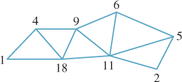
Figure 25.1: A triangle strip is represented by a stream of vertex indices; every group of three adjacent indices describes another triangle in the strip. The communication attributable to a typical triangle is therefore just a single vertex index, rather than three vertex indices.
At the abstract level—the mesh being represented—there’s no important difference between the full representation and the stripped or fanned representation. The choice of whether to use strips or fans depends on whether transmission of geometry (typically from a CPU to a GPU) is the primary bottleneck, or whether something else, like fill rate (the speed of converting triangles into pixel values), dominates.
In modeling, as opposed to rendering, today’s dominant technologies are splines (particularly NURBS) and quad-based subdivision surfaces; both of these are closely related to meshes. And in many application areas, including scientific visualization and medical imaging, nonmesh data structures like voxels or point-based representations dominate.
These preferred representations change depending on what kinds of data are at hand and on system properties such as memory size, memory bandwidth, bandwidth to the GPU, etc. Even now, voxel representations are being seriously considered by game developers, while work in scientific visualization has moved heavily toward meshes to make better use of GPUs. As with every other engineering choice described in this book, meshes will never be the universally right or wrong answer; they are just one more representation for your toolbox.
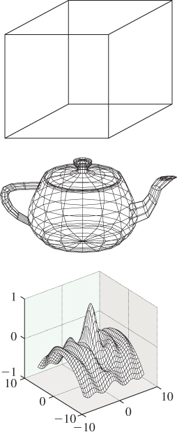
When we introduced meshes in Chapter 8, we did so as a means of representing geometry, like that shown in Figure 25.2. But there are other applications as well. Sometimes the vertex coordinates for a mesh are not physical locations, but instead are colors, or normal vectors, or even points in a configuration space (i.e., each vertex might describe a “pose” of a jointed figure; edges would then correspond to interpolations between poses, etc.).
The vertex-and-face-tables model of Chapter 8 appears to discount edges, which have no explicit representation. Nonetheless, faces are not all that matters. Edges are important in nonphotorealistic rendering, and in visibility-determination algorithms. Vertices are important in defining functions on meshes, as we discussed in Chapter 9. And most of all, connectivity is critical in many applications. The lack of explicit representation of connectivity or edges should not be taken as a mark of their unimportance.
The vertex-and-face-table representation could be enhanced with an edge-table representation; each row of the edge table would contain indices of two vertices that were to be joined by an edge. In this exercise, we’ll examine the consequences of introducing an edge table.
(a) Assuming that the edges in a mesh are exactly those that are part of the boundary of a face, describe an algorithm for deleting a face from a mesh.
(b) Suppose that edges are to be treated as directed, that is, the edge (3, 11) is different from the edge (11, 3), and that the same is true for faces. The boundary of the face (3, 5, 8) consists of the three directed edges (3, 5), (5, 8), and (8, 3). Assuming that we agree that the shapes we represent are all to be polygonal surfaces, discuss face deletion again. Make a Möbius strip from five triangles, and check whether your deletion algorithm works for the deletion of each triangle.
25.2. Mesh Topology
The topology of meshes—what’s connected to what—is of primary importance in many mesh algorithms, which often proceed by some kind of adjacency search like depth-first or breadth-first search. In this section we’ll discuss the intrinsic topology of meshes (i.e., those aspects that can be determined by looking only at the face table), and we’ll briefly touch on the topic of embedding topology for meshes that are embedded in 3-space (i.e., for which there’s a vertex table specifying positions of vertices, and for which the resultant mesh has no self-intersections, which we’ll define precisely).
To specify the topology of a triangle mesh, we typically choose a collection of vertices (usually represented by vertex indices, so we speak of vertex 7, or vertex 2), a collection of edges, with each edge being a pair of vertex indices, and a collection of faces, with each face being a triple of vertex indices. We’ll put additional constraints on these in a moment. Because a vertex consists of one index, an edge consists of two indices, and a face consists of three indices, it’s useful to have a term that encompasses all three. We say that a k-simplex is a set of k + 1 vertices. Thus, a vertex is a 0-simplex, an edge is a 1-simplex, and a face is a 2-simplex. (These ideas can be generalized to describe tetrahedral meshes, in which 3-simplices are allowed, and to even higher-dimensional meshes.)
The degree of a vertex is the number of edges that contain the vertex. The term valence is also used, by analogy with atoms in a molecule. The vertex is said to be adjacent to the edges containing it, and vice versa. We generalize to say that the degree of an edge is the number of faces that contain the edge. (The edge is said to be adjacent to the faces, and vice versa.) We’ll restrict our attention to meshes in which each edge has degree one, in which case it’s called a boundary edge, or degree two, in which case it’s called an interior edge (see Figure 25.3). An edge that’s adjacent to no faces at all is called a dangling edge and is not allowed in our meshes.

Figure 25.3: A small mesh with interior edges drawn in green and boundary edges drawn in blue. The red edge, which is not adjacent to any faces, is a “dangling” edge and is not allowed in our meshes.
25.2.1. Triangulated Surfaces and Surfaces with Boundary
To make our algorithms clean and provably correct, we will restrict the class of triangle meshes that we allow. We’ve already restricted our attention to meshes where each edge has one or two adjacent faces, but we will need some additional restrictions.
1. Each face may occur no more than once, that is, no two faces of the mesh can share more than two vertices.
2. The degree of each vertex is at least three.
3. If V is a vertex, then the vertices that share an edge with V can be ordered U1, U2, ..., Un so that {V, U1, U2}, {V, U2, U3}, ..., {V, Un–1, Un} are all triangles of the mesh, and
(a) {V, Un, U1} is a mesh triangle (in which case V is said to be an interior vertex), or
(b) {V, Un, U1} is not a mesh triangle (in which case V is said to be a boundary vertex),
and there are no other triangles containing the vertex V (see Figure 25.4).
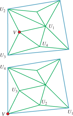
Figure 25.4: The red vertex marked with a dot in the top mesh is an interior vertex; the one in the bottom mesh is a boundary vertex.
In the event that such a mesh has no boundary vertices, it’s called a closed surface; if it has boundary vertices, it’s called a surface with boundary.
Figure 25.5 shows three surfaces, each of which fails the requirements for being a surface or surface with boundary. Explain the three failures.
We have not yet said anything about orientation or orientability so that, for instance, the Möbius band is a perfectly admissible surface with boundary.
Show that the mesh with faces (1, 2, 3), (2, 3, 4), (3, 4, 5), (4, 5, 1), (5, 1, 2) and vertices 1, 2, 3, 4, and 5 is a surface with boundary (i.e., satisfies all the conditions above). Determine the set of boundary edges.
The boundary of a simplex is gotten by deleting each vertex of the simplex in turn, so the boundary of {2, 3, 5} consists of the three sets {2, 3}, {2, 5}, and {3, 5}. Similarly, the boundary of the 1-simplex {2, 4} consists of the two sets {2} and {4}. The boundary of the 0-simplex {8} consists of the empty set.
25.2.2. Computing and Storing Adjacency
The basic mesh-storage structure is the face table, but adding and removing faces from an array is slow. Storing faces in a linked list rather than a table represented as a matrix allows low-overhead addition and deletion of faces, but operations like detecting adjacency can be expensive. The winged-edge data structure described in Chapter 8 makes adjacency computations very quick, but addition and deletion are relatively heavyweight operations.
Most adjacency-determining operations can be done, in a precomputation step, with hash tables. For instance, here’s how to determine all boundary edges: First, for any face like {5, 2, 3}, there are three edges, each of which we’ll represent with an ordered pair. But the first edge could be represented by the pair (2, 5) or (5, 2). We’ll make the choice of representing the vertices in an edge in increasing order, so the edges are (2, 5), (3, 5), and (2, 3). With this convention, finding the boundary edges is easy: We start with an empty hash table of edges. For each face of the mesh we compute the three edges, and for each such edge we either insert it in the table if it’s not there already or delete it from the table if it is there already. When we’ve processed all the faces, the edges that remain in the table are those that appeared only once; in other words, they are the boundary edges.
The boundary-finding algorithm above assumed that the mesh was a closed surface or a surface with boundary, that is, it satisfied all the conditions for being a surface. Think about how you could use a similar algorithm to determine that the mesh did indeed satisfy all these conditions. Condition 3, which characterizes interior and boundary vertices, is a bit tricky, and you can skip that one if you like.
Our definition of a surface was quite general, but in practice most of the surfaces we meet in graphics are orientable, or even oriented. To define an oriented surface we need the notion of an oriented simplex: An oriented simplex is not just a set, but an ordered set. A 0-simplex is still just a vertex. A 1-simplex is an ordered pair (i, j) of distinct vertex indices. And a 2-simplex is an ordered triple (i, j, k) of distinct vertex indices, with the convention that (i, j, k), (j, k, i), and (k, i, j) are all considered “the same.” (Alternatively, one can make the convention that the lowest-numbered vertex is always listed first; the order of the remaining two vertices determines the orientation of the face.)
The (oriented) boundary of an oriented face is built by deleting one vertex at a time, and reading the others in cyclic order, so the oriented boundary of the oriented face (2, 5, 3) consists of the oriented edges (2, 5), (5, 3), and (3, 2).
For a mesh to be oriented requires that the faces be oriented simplices, and that if vertices i and j of edge e are contained in two distinct faces f1 and f2, then they must appear in the order (i, j) in one of them and (j, i) in the other.
An oriented face is often drawn symbolically with a small arrow indicating the orientation, that is, the cyclic order of the vertices. Figure 25.6 shows an example of two adjacent faces—the edge (3, 7) appears in the first; the edge (7, 3) in the second.
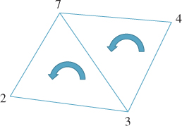
Figure 25.6: Two oriented adjacent faces, (2, 3, 7) and (7, 3, 4). The oriented edge (3, 7) is in the boundary of the first face, while (7, 3) is in the boundary of the second.
If we are given the face table for a connected unoriented mesh, we can try to create an oriented mesh from it: We take the first triangle, say, {2, 6, 5}, and assign it an order, say, (2, 5, 6). We then seek out an adjacent face, say, (9, 2, 5), and since it shares the vertices 2 and 5 with the first face, we have to place them in the opposite order, that is, we assign the order (9, 5, 2). We continue in this fashion, assigning an order to each face adjacent to those already assigned, following either a depth-first or breadth-first strategy. If we encounter a face that’s already been oriented, we check to verify that the orientation is consistent with the current face (i.e., it’s the orientation we’d have assigned if it weren’t already done!). If it’s consistent, we ignore the face and continue; if it’s inconsistent, we terminate the algorithm and report that the mesh is not orientable.
(a) Describe how to determine whether a mesh is connected (i.e., whether the graph consisting of all vertices and edges of the mesh is a connected graph).
(b) Apply the orientation algorithm to the five-vertex mesh of Inline Exercise 25.3 to show it’s not orientable.
(c) Once we orient one face of an orientable connected mesh, all others have their orientations determined by the algorithm just described, so there are only two possible orientations of any connected orientable mesh. Suppose that some mesh M is not connected, and instead has n > 1 components. How many different orientations can it have?
The algorithm above can be slightly modified to compute the oriented mesh boundary: In the course of processing each face, if one of its edges is not part of a second face, we record that (oriented) edge as part of the oriented boundary.
Although we’ve described orientable meshes and an algorithm for determining an orientation (i.e., a consistent orientation for each face), in practice we usually encounter oriented meshes, or ones for which a particular orientation has already been chosen. When these meshes represent closed surfaces in 3-space, like a sphere or torus, the orientation of a face (i, j, k) is usually chosen so that if v1 is the vector from vertex i to vertex j, and v2 is the vector from vertex j to vertex k, then v1× v2 points “outward,” that is, toward the unbounded portion of space.
Current work in collision detection primarily uses oriented meshes, and often stores triangles as lists of edges (or along with lists of their edges). The reason has to do with speeding up certain tests that occur often, namely, point-in-triangle tests. If you have a point P in the plane of a triangle ABC in space, and you want to test whether it’s actually within the triangle, you can do three “Is this point on the right side of this plane?” tests to answer the question. Here’s how: Let’s suppose that the plane of ABC is S. Consider any plane J that contains the edge AB and is not parallel to S (see Figure 25.7). The plane J can be characterized by a point Q on the plane and a normal vector n; the equation for J is then
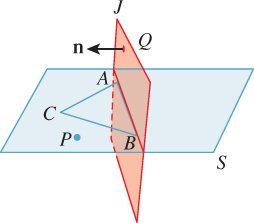
Figure 25.7: The point P is on the same side of the plane J as C, and therefore may be in the triangle ABC. If it passes corresponding tests for planes containing the edges BC and CA, we know it’s in the triangle.
To determine whether P is on “the right side” of J, we can substitute C for X in Equation 25.1; the result will be nonzero. If it’s negative, we’ll replace n by –n, so we can assume that it’s positive:
Now that we’ve arranged for n to point in the proper direction, the test for P being on the right side of J becomes
If we compute Q and n once, we can associate them to the edge AB and reuse them for every point-in-triangle test.
The point-versus-plane test involves a point subtraction, a dot product, and a comparison. Assuming that all points are stored as triples of coordinates, we can consider the special point Z = (0, 0, 0) and rewrite the test as ((P – Z) – (Q – Z)) · n > 0, or (P – Z) · n > (Q – Z) · n. Assuming that this computation appears in the innermost loop of your program so that you’re willing to ignore the point-versus-vector distinction, and assuming further that you’re willing to do more precomputation, how few operations can you use to do this computation for each new test point P? (Answer: three multiplies, two adds, one compare. Your job is to verify this.)
One final data structure for meshes—and one that is particularly useful for meshes that will remain mostly topologically static, that is, for which addition and removal of faces is very rare—is an enhancement of the triangle mesh in which row i of the face table stores the indices of the three vertices for triangle i, but also stores the indices of the three triangles that are adjacent to triangle i. (If triangle i has one or two edges on the boundary of the mesh, then the corresponding index is set to invalid.) This structure speeds up coherent searching of the mesh data structure, especially for processes like contour finding. (If edge e is a contour edge as seen from some viewpoint, then the edges that meet e are very good candidates to also be contour edges.)
There are analogous structures for quad meshes. The difference between triangles and quads may seem small, but it’s nontrivial. If you can replace a pair of adjacent triangles with a quad, you’ve turned five edges into four, and that may mean a 20% speedup in your program.
25.2.3. More Mesh Terminology
The star of a vertex consists of the vertex itself and the set of edges and faces that contain that vertex (i.e., like a “neighborhood” of the vertex). The star of an edge consists of the edge itself and any faces that contain the edge. Figure 25.8 shows the star of a red vertex in red tones and the star of a green edge in green tones. The link of a vertex is the boundary of the star. Suppose V is a vertex in a closed mesh. Each vertex in the link of V is separated from V by a single edge. These vertices are therefore called the 1-ring of V; those separated by a distance of two edges are called the 2-ring (see Figure 25.9). The vertices of the 1-ring of an interior vertex can always be organized into a cycle; that follows from the definition of a surface mesh. For the 2-ring, bad things can happen. For instance, in a tetrahedron, the 2-ring of any vertex is empty; in an octahedron, the 2-ring of any vertex is a single vertex. Figure 25.10 shows a mesh in which the 1-ring of a vertex is nice, but the 2-ring forms a figure-eight shape.
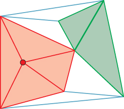
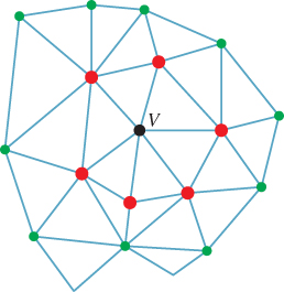
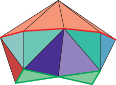
Figure 25.10: The star of the top vertex is drawn in brown; the 1-ring, which forms an octagon in the middle level, in red. The 2-ring, at the bottom drawn in bright green, is connected into a figure-eight shape.
When we compute the boundary of a mesh, the boundary edges form chains; each such chain is called a boundary component, and the number of boundary components is often denoted by the letter b.
If a mesh surface M has v vertices, e edges, and f faces, the number χ = v – e + f is called the Euler characteristic of M, and it measures the “complexity” of the surface: A spherical topology has characteristic 2; a torus has characteristic 0; a two-holed torus has characteristic –2; and in general, an n-holed torus has characteristic χ = 2 – 2n. If the n-holed torus also has b boundary components, then the formula becomes χ = 2 – 2n – b.
25.2.4. Embedding and Topology
When we assign locations to the vertices of a surface mesh (and to the rest of the mesh by linear interpolation), we want the resultant shape to resemble a surface that has an interior and an exterior, and no self-intersections. To distinguish between the abstract surface mesh (a list of vertices numbered 1, ..., n, and a list of “faces,” or triples of vertex indices) and the geometric object associated to it, we’ll use lowercase letters like i and j to indicate vertex indices, and Pi and Pj to indicate the geometric locations of vertices i and j. We’ll also use C(Pi, Pj) to denote all convex combinations of Pi and Pj, that is, the (geometric) edge between them, and C(Pi, Pj, Pk) to denote all convex combinations of the vertex locations Pi, Pj, and Pk, that is, the (geometric) triangle with those points as vertices.
With this terminology, we’ll define an embedding of a surface mesh as an assignment of distinct locations to the vertices, extended to edges and faces by linear interpolation and satisfying one property: The triangles T1 = C(Pi, Pj, Pk) and T2 = C(Pp, Pq, Pr) intersect in R3 only if the vertex sets {i, j, k} and {p, q, r} intersect in the abstract mesh. If the intersection is a single vertex index s, then T1 ![]() T2 must be Ps; if the intersection has two vertices s and t, then T1
T2 must be Ps; if the intersection has two vertices s and t, then T1 ![]() T2 = C(Ps, Pt); and if the intersection is all three vertex indices, then T1 must be identical to T2. (Note that we’re assuming that i, j, and k are distinct and p, q, and r are distinct; otherwise, either T1 or T2 would not be a triangle.)
T2 = C(Ps, Pt); and if the intersection is all three vertex indices, then T1 must be identical to T2. (Note that we’re assuming that i, j, and k are distinct and p, q, and r are distinct; otherwise, either T1 or T2 would not be a triangle.)
Figure 25.11 shows examples of nonembedded meshes. In the first example, two triangles intersect in their interiors. In the second, two triangles intersect at a point that is a vertex of one triangle, but is mid-edge on the other triangle. In the third, the intersection (shown in aqua) of two shaded triangles is only part of an edge of the left one (a situation known as a T-junction).
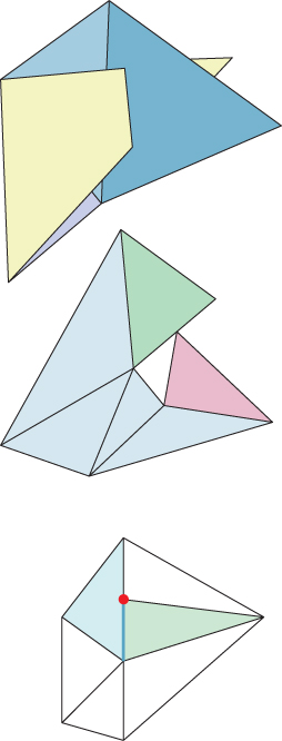
Figure 25.11: (Top) A mesh with bad self-intersections. (Middle) A mesh in which a vertex of the pink face at the right lies in the middle of an edge of the green face at the top right. (Bottom) The red vertex marked with a dot is a T-junction.
When we have both a face table and a vertex table, we can test whether the resultant geometric mesh is embedded or not, but the operation is expensive and prone to numerical errors. First, the entries of the vertex table (i.e., the vertex locations) must all be distinct. Second, for every pair of faces the geometric intersection of the faces must be empty unless the abstract faces share an edge or a vertex, in which case the geometric intersection should match the abstract intersection. Good modeling software is designed to ensure that only embedded meshes get produced so that such tests are not necessary.
If a mesh is closed, that is, its boundary is empty, and if it’s embedded, then (1) the mesh must be orientable, and (2) the embedded mesh divides 3-space into two parts: a bounded piece called the interior and an unbounded piece called the exterior. The first statement is proved by Banchoff [Ban74]; the second, which may seem obvious, is really quite subtle, and is a consequence of the Alexander Duality Theorem [GH81], which is far beyond the scope of this book. To determine whether a point P that’s not on the mesh itself is in the interior or exterior, we can create a ray r that starts at P and travels in some direction d, missing all vertices and edges of the mesh. If the ray r intersects k faces of the mesh, then P is inside if k is odd and outside if k is even. The direction d can be produced by picking a direction at random; with probability one the ray r will miss all vertices and edges of the mesh.
A closed embedded mesh is, from a geometric and algorithmic point of view, an ideal object. It’s suitable for use in ray tracing, in rendering with backface culling, for shadow-volume computations, etc. Furthermore, if a closed mesh is embedded and we move the vertex locations by a small enough amount, the resultant mesh is still embedded. “Small enough” in this case means “less than ε/2, where ε is the smallest distance from any vertex to any other vertex, or to the edge between any two other vertices, or to the plane containing any other three vertices, or from any edge to any nonintersecting edge of the mesh.
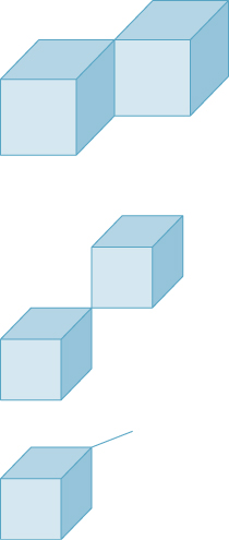
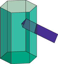
A closed, embedded surface mesh is sometimes called a watertight model, although it’s possible to have a model that’s intuitively “watertight” without satisfying the definitions for closed-ness, surface-ness, and embedding. As a simple example, a cube that has an additional square dividing it into two half-cubes is “watertight,” in the sense that water placed in either of the two “rooms” can’t escape, but it fails the tests of “surface-ness” and embedding. At a more practical level, it can be convenient to create a video-game model of, say, a robot character in which the torso is a polygonal cylinder (with endcaps) and the upper arm is an open-ended triangular prism that goes through the torso (see Figure 25.12). Clearly no water can leak from the torso into the upper arm, and this structure makes it easy to adjust the arm position over some range without worrying about things matching up perfectly.
On the other hand, while modeling and animating the character with this approach is easy, rendering it, or creating shadows from it, may be quite difficult. The same goes for models containing T-junctions.
25.3. Mesh Geometry
From now on, we’ll assume we’re working with embedded oriented surface meshes, although not necessarily closed meshes—there may be boundary components.
We’ve suggested that surface meshes are the discrete analog of smooth surfaces, but there are subtleties. On a smooth surface, for instance, at each point P there’s a tangent plane that approximates the surface near P: In a small enough region around P, projection from the surface to the tangent plane is injective, that is, no two points in the neighborhood project to the same place on the tangent plane. Figure 25.13 shows this for the sphere. By contrast, there are quite simple meshes for which there is no such plane. Figure 25.14 shows an example of a vertex with the property that no plane passing through it will serve as a “tangent plane”; projection in any direction is never injective.
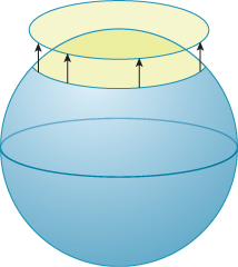
Figure 25.13: In this simple model of Earth, a small disk around the North Pole projects injectively onto a disk in the horizontal tangent plane to the North Pole.
The situation shown in Figure 25.14 may seem pathological, but it can arise quite easily during the gluing together of points obtained from a surface by scanning. A vertex like the one in the figure is said to be “not locally flat”; a locally flat vertex P is one for which there’s a vector n such that projection from the star of P onto the plane through P with normal n is injective. Generally speaking, vertices that are not locally flat tend to break algorithms; it’s a good idea to check that the vertex normal n assigned to each vertex P of a mesh demonstrates the local flatness property at P.

Figure 25.14: Projection from the mesh onto any plane passing through the central red vertex will not be injective. The large green vertices are closer to the eye; the small aqua ones are farther away.
The local flatness example demonstrates a general phenomenon: Things that you know about smooth surfaces don’t directly apply to meshes. For instance, the slices perpendicular to some generic direction d of a smooth surface tend to be nice, smooth curves, except at isolated “critical” points, where there may be self-intersections that look like the letter X, as shown in Figure 25.15. By contrast, the slices of a surface mesh are polygonal curves, and at critical points they can look very complicated indeed [Ban65].
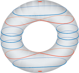
Figure 25.15: The slices of a torus are smooth (blue) except at the min, max, and the two “critical” levels where the slices are figure-eights (red).
As another example, the contours of a smooth surface, that is, the points where the view ray lies in the tangent plane, generally form a set of smooth, closed curves on the surface, curves that don’t intersect one another. For instance, the contour of a sphere is always a circle on the sphere’s surface. For some surfaces, from some points of view, the contours may have intersections or sharp corners, but from a randomly picked direction they will be smooth. By contrast, the contours of a closed triangulated mesh consist of edges that lie between front-facing and back-facing polygons. These contours are therefore polygonal rather than smooth curves. But as Figure 25.14 shows, the polygonal curves may intersect, and may do so generically (i.e., there’s a nonzero probability that for a randomly chosen direction such problems occur).
To the degree that we treat triangulated meshes as surfaces in their own right, rather than as approximations of smooth surfaces, these oddities are hardly surprising. In a mesh, almost all points are flat: The curvature, no matter how you measure it, is zero. On the other hand, the curvature along edges or at vertices is, by the usual measures, infinite. It’s as if the curvature that was spread out over a smooth surface got “condensed” into tiny packets of high curvature. All the techniques of differential geometry, which depend on taking derivatives of a parameterization of the surface, must be rethought in this context. The resultant discrete differential geometry is an active area of research [Ban65, BS08].
25.3.1. Mesh Meaning
In Figure 25.2, the cube has sharp edges and is intended to be a sharp-edged shape. By contrast, the wavy surface does have a bend at each edge, but the bend is very small, and the intent is that it should be seen as a smooth shape. When you work with a mesh in a graphics program, you don’t generally know which one of these is intended. Expressed differently, you know the data for the mesh, but you don’t know what it means. Just as RGB image formats that fail to say what R, G, and B mean can have many interpretations (see Chapter 17), meshes that don’t include a description of their meaning are ambiguous, and any single interpretation you choose in writing a program will be wrong in some cases. This is an example of the Meaning principle: The numbers (and other data) used to represent meshes don’t have enough meaning to be unambiguous, and this failure of meaning leads to failed algorithms.
For the bulk of this chapter, we’ll assume that meshes are being used to approximate smooth surfaces, thus assigning a meaning to each mesh. In Chapter 6, we saw how this assumption can lead to problems. The pyramid looked odd until we remade it from several different meshes. But this remaking entailed its own problems: To make the pyramid taller now requires that we move not a single vertex, but several copies of that vertex. The important topological structure was broken in order to provide a correct rendering structure. For instance, although the original pyramid might have been a watertight mesh, the new pyramid is not. That’s partly a consequence of the design of graphics interfaces. For instance, both OpenGL and DirectX require that all the properties of a vertex, such as its normal vector and texture coordinates, be tied to the vertex position in an indexed triangle strip. If you want to make a shape like a cube, where a single vertex must have multiple normal vectors, you’re compelled to create multiple vertices at the same location, leading to nonwatertight models. And all current hardware APIs specify properties either at the per-mesh level or at the per-vertex level, so concepts like face color have to be implemented by a similar vertex-duplicating strategy in which all three vertices of a face are assigned the same color, requiring multiple co-located vertices and nonwatertightness of the meshes.
As you think about applying any particular algorithm to your own meshes, be sure that your assumptions about the mesh and those made by the algorithm designer actually match, or expect bad results.
25.4. Level of Detail
A model of an office building might contain millions of polygons, both for interior detail and for things like windows, frames, exterior trim, etc. If that building is to appear in the far distance in some scene, it may suffice to remodel it as a single rectangular box. Indeed, if you do not remodel it that way, then rendering just a few city blocks will rapidly consume your entire budget for polygons, while perhaps only determining the final appearance of a small fraction of the pixels in your image. This is a clear misallocation of resources. If you’re using basic z-buffering to determine visibility, and your building occupies, say, 100 pixels of the image, then (since each pixel’s color is determined by the frontmost polygon drawn in it) all but 100 of your 1 million polygons will have been drawn to no avail.
It’s possible to improve this situation substantially with visibility hierarchies so that, for instance, none of the polygons interior to your building get drawn. But for a building with substantial exterior detail, this is merely a palliative measure. What’s really needed is a different model of the building, used when the model is in the distance. If you make an animation, the high-detail model is used when the building is nearby and the low-detail model is swapped into its place as the building recedes into the distance. Naturally, it’s important that the swapping process be relatively undetectable, or the illusion of the animation will be broken. The substitution of a simpler model for the completely detailed model can be done in stages; in other words, it makes sense to build a model that includes multiple levels of detail, each one used where appropriate.
The inclusion of levels of detail represents a substantial architectural shift. Normally we imagine a renderer asking each object for a polygonal representation of itself, and then producing an image from these polygons. In a system using level of detail, the renderer must ask the object for a polygonal representation and provide some information about the level of detail. This information might be something like the distance from the camera to the object’s center, or a request for the object to provide a representation with no more than 10,000 polygons, or a request to provide one of three or four standard levels of detail.
I can render a building from nearby with a wide-angle lens; the building fills most of the image. I can render it from very far away with a narrow-angle lens, and again it fills most of the image. What does this suggest to you about using the distance to the object as a level-of-detail cue? What might improve it?
A useful approach for determining level of detail is to have a coarse representation of the model, such as a bounding box; the rendering software can then quickly determine the screen area of the bounding box, and it can use this to help the object select the appropriate level of detail. In expressive rendering (see Chapter 34), we sometimes elide detail on an object for reasons other than screen size (e.g., we might draw the details on only one or two faces in a crowd, because they are the important ones); in such a case, the level-of-detail negotiation between renderer and object may include hints other than the purely geometric ones discussed here.
While we’ve described level of detail here as a solution to a resource-allocation problem, it is more than that: Once we have decided to produce a final image using a single-sample z-buffer technique (or any other approach that uses a small, fixed number of samples per pixel), we’ve implicitly settled on a “scale” for which we can hope to produce correct results. Assuming, for the sake of argument, one sample per pixel, any geometric feature—a step, a windowsill, a doorknob—whose projected size is less than two pixels will produce aliasing instead of being accurately reconstructed. Because of this, we’d like to remove all such features, in a sense “prefiltering before sampling.” Thus, using a level-of-detail approach is a matter of correctness as well as efficiency. We summarize these ideas in a principle:
![]() Level of Detail Principle
Level of Detail Principle
Level of detail is important for both efficiency and correctness.
That being said, the “correctness” provided by level-of-detail simplifications is not always all that one might wish. Consider the front of a building shown in Figure 25.16. The natural “simplification” of this wall is to replace it with a single planar wall.
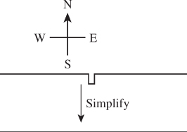
Figure 25.16: The front wall of a building, seen from above. Notice the narrow embossed portion of the wall in the center. The sides of this embossment will reflect light from the east or west, while the rest of the wall will not.
But now consider the light-reflection properties of these two versions of the building’s front. If we assume that the front of the building is made of a somewhat glossy material, then in the unsimplified wall, some light from the east will reflect back toward the east, and some light from the west will reflect back to the west, while lots of light from the south will reflect back toward the south. The bidirectional reflectance distribution function (BRDF) of the wall as a whole, for three incoming light directions, is shown in Figure 25.17. The BRDF for the simplified wall is rather different, since it’s everywhere zero for light from the east, for instance.
We could, as we simplified the wall, still represent the geometry by encoding it in a normal map. But as we decrease the level of detail on the building further, the normal map itself will have to be simplified as well, to avoid representing too-high frequency changes. At that point, we can amalgamate the different reflection characteristics of the surface at different points into a single BRDF that resembles the “various facets in the wall look a lot like the microfacets” concept used in the Torrance-Sparrow and Torrance-Cook models, in the sense that they are geometric features that are too small (in screen coordinates) for us to detect, and hence we aggregate their effects into a BRDF.
We saw this sort of thing before, back in Chapter 18: If we’re taking samples from a function in hopes of saying something about it, then our sampling rate should exceed the Nyquist rate for the signal, or we’ll suffer aliasing. In this case, the “function” could be either “the x (or y or z)-coordinate of the points on the surface,” or “the BRDF of the surface” (considered as a function of position on the surface), or “the color of the surface,” etc.
In fact, many of the techniques we’ve encountered—BRDFs, normal maps, displacement maps—provide representations of geometry at different scales. The BRDF (at least in the Torrance-Sparrow-Cook formulation) is a representation of how the microfacet slope distribution affects the reflection of light from the surface. We could model all those microfacets, but the space and time overhead would be prohibitive. More important, the result of sampling such a representation (e.g., ray-tracing it) would contain horrible aliases: A typical ray hits one particular microfacet and reflects specularly, rather than dispersing as we’d expect for a diffuse reflection. Displacement maps and normal maps represent surface variation even for surfaces that are, at a gross scale, represented by just a few polygons. Because of their formulation as maps (i.e., functions on the plane), they can be filtered to reduce aliasing artifacts, using MIP mapping, for example.
Fortunately, these techniques also constitute a hierarchy of sorts: As you simplify one representation, you can push information into another. A crinkled piece of aluminum foil, for instance, can be modeled as a complex mesh with a very simple (specular) BRDF, if it’s seen close-up. As it recedes into the distance, we can replace the complicated geometry with a simpler planar polygon, but we can represent the “crinkliness” by a normal map and/or displacement map. As it recedes farther into the distance, and variations in the normal map happen at the subpixel scale, we can use a single normal vector, but change the BRDF to be more glossy than specular, aggregating the many individual specular reflections into a diffuse BRDF. Many of these ideas were present (at least in a nascent form) in Whitted’s 1986 paper on procedural modeling [AGW86].
The correspondence with the sampling/filtering ideas is more than mere analogy: In rendering, we’re trying to estimate various integrals, typically with stochastic methods that use just a few samples; from these samples, we implicitly reconstruct a function in the course of computing its integral. If the function is ill-represented by the samples, aliasing occurs. In one-sample-per-pixel ray tracing, for instance, any model variation that occurs at a level that’s smaller than two pixels on the screen must either (a) be filtered out, or (b) appear as aliases.
In some sense, these observations give an abstract recipe for how you ought to do graphics: You decide which radiance samples you’ll need in order to represent the image properly, and then you examine the light field itself to determine whether taking those samples will generate aliases. If so, you determine what variation needs to be removed from the light field; since the light field itself is determined by the rendering equation, you can then ask, “What simplification of the illumination or geometry of this scene would remove those problems from the light field?” and you remake the model accordingly. When you set about rendering this model, you get the best possible picture.
This “recipe” is an idealized one for several reasons. First, it’s not obvious how to simplify geometry and illumination to remove “only the bad stuff” from the light field; indeed, this may be impossible. Second, determining the “bad stuff” in the light field may require that you solve the rendering equation with the full model as a first step, which returns you to the original question. A compromise position is that if we filter the light sources to not have any high-frequency variations, and we smooth out the geometry so that it doesn’t have any sharp corners (which lead to high-frequency variations in reflected light), then the “product” of light and geometry represented by the rendering equation will end up without too much high-frequency information in it. While this loose statement may be correct, it’s not the case that the smoothed lighting of smoothed objects produces the same result as taking full-detail lighting of the full-detail model and smoothing the results. The “smoothing” operation (filtering out high frequencies) does not commute with the “product” operation in the rendering equation (another instance of the Noncommutativity principle). Then again, it’s the best we’ve got at present, and it’s an approach that forms the basis for many techniques.
Before leaving this high-level discussion, we have two more observations. The first is that, in thinking about graphics, we tend to think about the kinds of models being used to represent the world, and it’s easy to confuse the “nature of the world” with the “nature of models representing it.” As three points on the continuum of model classes, consider (a) tessellation-independent models, like the implicit surfaces used in making a simple ray tracer, (b) collections of triangles and/or “primitives” like cubes, spheres, cones, spline patches, etc., combined with unions, intersections, etc., to describe shapes, and (c) “object-based” graphics, in which the world is populated by objects, each one modeled in its own way and each one supporting various operations like “Where does this ray intersect you?” and “Give me a simplified representation of yourself.” If objects are themselves represented as meshes (as they often are), it’s very natural to ask, “What’s a simplified representation of this object?” to do level-of-detail computations at a per-object level. The problem with this approach is that the result of simplification depends on our description of the world, not the world itself. For instance, if we have a sphere that’s represented by an icosahedral mesh, it’s natural to simplify it by replacing that mesh with an octahedron or tetrahedron. But if we happen to have created that same shape with 20 objects, each of them a single triangle, then there’s no possible simplification: Each triangle is as simple as can be. To give another example, if we have two irregularly shaped objects partly overlapping each other (see Figure 25.18), and we simplify each of them to remove fine detail, the gap between them can remain as a small detail, and hence a source of aliasing when we sample the scene. This happens in practice when we model a city as many buildings: Even when all the buildings are simplified to cuboids, the spaces between them may be rectangular gaps that are so small, in screen space, that they produce aliases.
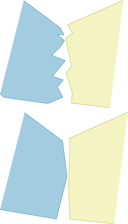
Figure 25.18: Two irregularly shaped objects overlap; when we simplify each one, getting rid of small details, the space between the objects remains as a small detail, unrecognized by our simplification process.
One approach to level of detail is therefore to consider the simplification of a whole scene at a time. Perbet and Cani [PC01] took this approach in modeling prairies: Grass near the camera was modeled as individual blades; slightly more distant grass was represented by flexible vertical panels on which the blades of grass were “painted.” And very distant grass was represented by textures applied to large horizontal planar polygons. The intermediate representation—a textured polygon that faces the viewer—is one instance of a billboard. Numerous permutations of this billboard idea have been used over the years, from representing trees by an intersecting pair of billboards (which looks decent, except when viewed from above), to increasingly complex combinations such as the representation of clouds by multiple semi-transparent billboards [DDSD03], to the representation of crowd characters by billboard assemblies with time-varying textures [KDC+08].
One very natural approach to level of detail is to represent the world (or an object) as a union of spheres. Simplification is natural: One replaces several small spheres with a larger sphere that encloses (partially or completely) the small ones. Such representations are easy to translate and rotate, and spheres are simple enough that they’re amenable to lots of algorithmic tricks that make the construction of sphere trees [Hub95] relatively easy. This line of work goes back to Badler [BOT79].
One final class of objects deserves mention in the context of level of detail: parametric curves and surfaces. In these cases, the coordinate functions t ![]() (x(t), y(t), z(t)) or (u, v)
(x(t), y(t), z(t)) or (u, v) ![]() (x(u, v), y(u, v), z(u, v)) are real-valued functions, typically defined on an interval or rectangle. As such, they’re amenable to Fourier analysis (representation as sums of sines and cosines), and hence to filtering. In specific cases (like B-splines), there are other approaches to simplification, such as replacing a B-spline by its control-point polygon. And in other cases, bases other than the Fourier basis may be appropriate: Finkelstein et al. [CK96] represented level of detail in a B-spline wavelet basis, which allows for both simplification (by eliminating detail beyond a certain scale) and multiscale editing (see Figure 25.19); there are similar approaches for wavelet representations of surfaces [ZSS97] to allow multiscale editing and simplification.
(x(u, v), y(u, v), z(u, v)) are real-valued functions, typically defined on an interval or rectangle. As such, they’re amenable to Fourier analysis (representation as sums of sines and cosines), and hence to filtering. In specific cases (like B-splines), there are other approaches to simplification, such as replacing a B-spline by its control-point polygon. And in other cases, bases other than the Fourier basis may be appropriate: Finkelstein et al. [CK96] represented level of detail in a B-spline wavelet basis, which allows for both simplification (by eliminating detail beyond a certain scale) and multiscale editing (see Figure 25.19); there are similar approaches for wavelet representations of surfaces [ZSS97] to allow multiscale editing and simplification.
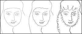
Figure 25.19: A curve, represented in a wavelet basis, consists of large- and small-scale features. The small-scale features—the “character” of the curve—can be edited without affecting the large-scale shape, and vice versa. (Courtesy of Adam Finkelstein and David H. Salesin, ©1994 ACM, Inc. Reprinted by permission.)
25.4.1. Progressive Meshes
From these generalities, we’ll now move on to a specific algorithm for mesh simplification, Hoppe’s progressive meshes. The goal of progressive meshes is to start from a mesh Mn of n nodes, and simplify it to a mesh of n – 1 nodes by collapsing one edge (thus merging two adjacent nodes), as shown in Figure 25.20. The resultant mesh is denoted Mn−1. Successive collapses of edges lead to a sequence of meshes with fewer and fewer nodes, ending at M1, which consists of a single node. This provides a “continuous” level-of-detail representation for the mesh. Furthermore, the change from Mn to Mn−1 can be interpolated, in the sense that if we define ![]() to be a mesh with the topology of Mn, but with geometry modified so that the position ut of u is ut = (1 – t)u + tw, and similarly for v, then
to be a mesh with the topology of Mn, but with geometry modified so that the position ut of u is ut = (1 – t)u + tw, and similarly for v, then ![]() consists of exactly the same set of points as Mn–1; to convert one to the other requires deleting two area-zero triangles, and renaming some vertices and edges. This interpolation (see Figure 25.21) is called a geomorph (for “geometry morph”).
consists of exactly the same set of points as Mn–1; to convert one to the other requires deleting two area-zero triangles, and renaming some vertices and edges. This interpolation (see Figure 25.21) is called a geomorph (for “geometry morph”).
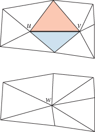
Figure 25.20: The edge from u to v has been collapsed to a single new vertex, which is labeled w. The two triangles that meet this edge have disappeared, and the four non-uv edges have collapsed into two edges. The set of triangles shown is called the neighborhood of the edge.
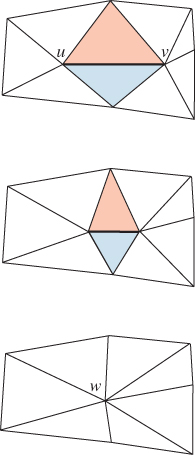
Figure 25.21: An edge-collapse can be made gradually, by interpolating from the original positions of u and v part of the way toward the final position w.
To complete the description of the algorithm, we need to know
1. How to choose a location for the new vertex w
2. How to choose, at each stage, which edge to collapse
For item 2 in the preceding list, Hoppe associates a cost (described below) to each possible edge collapse, and chooses the one with least cost (i.e., he pursues a greedy algorithm).
For item 1 in the list, Hoppe considers three possible locations for w: u, v, and ![]() . Each choice results in a different edge-collapse cost, and he chooses the one with the least cost.
. Each choice results in a different edge-collapse cost, and he chooses the one with the least cost.
25.4.1.1. Edge-Collapse Costs
To describe the cost of an edge collapse, we first need to describe how to measure how well a given mesh M fits a set of data X = {xi ![]() R3 : i = 1, 2, ..., N}. We’ll use a bunch of points from the original mesh Mn as the set X, but for now, you can imagine that Mn is a nice enough mesh that we can just use its collection of vertices as X. For the rest of this discussion, we’ll treat the set X as fixed, and not mention it explicitly.
R3 : i = 1, 2, ..., N}. We’ll use a bunch of points from the original mesh Mn as the set X, but for now, you can imagine that Mn is a nice enough mesh that we can just use its collection of vertices as X. For the rest of this discussion, we’ll treat the set X as fixed, and not mention it explicitly.
The goodness-of-fit is described by an energy, a function that measures how efficiently the mesh M approximates Mn as a sum of several terms,
where, for now, we’ll combine the last two terms into one,
which we can ignore for the time being. The “distance” term in the energy is the sum of the squared distances from each xi to M: For each xi, we find the closest point of M (which is itself a minimization problem), square it, and sum up the results. The “spring” term corresponds to placing a spring along each edge of the mesh M; the rest length of the spring is zero, so the total energy is
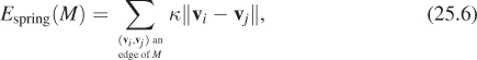
where κ is a spring constant that we’ll describe in a moment. The idea is to adjust the vertex locations for the mesh M to minimize this energy, thus finding a mesh that fits the data (X) well, while not having excessively long edges. Figure 25.22 shows why the spring-energy term is needed.
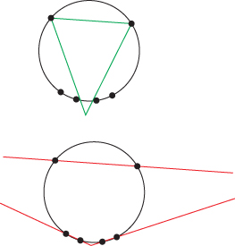
Figure 25.22: The value of “spring” energy: If we try to fit the six data points on a circle (marked with small dots) using a triangle with short edges, the green triangle (top) is a reasonably good solution. If we remove the short-edge constraint, the red triangle (bottom) is a “perfect” fit, even though it violates our expectations.
The cost of an edge collapse from a mesh M to a mesh M′ is determined by computing
which will generally be positive (it’s harder to fit the data with fewer vertices!). Of course, this cost depends on knowing the vertex locations for M′. Since the change from M to M′ is a single edge collapse, the new knowledge amounts to just the location of the vertex corresponding to the collapsed edge, since all other vertices remain unchanged. As we said, Hoppe restricts the possible new vertex locations for the edge between v1 and v2 to three choices: v1, v2, and their average. To compute the distance plus spring cost, he uses an iterative approach, which we sketch in Listing 25.1.
Listing 25.1: Finding the optimal placement of a vertex for a collapsed edge.
1 Input: a mesh M and an edge vsvt of M to collapse
2 Output: the optimal position for ![]() , the position of
, the position of
3 vertex s after the collapse
4
5 E ← ∞
6 repeat until change in energy is small:
7 Compute, for each xi ![]() X, the closest location bi on the
X, the closest location bi on the
8 mesh M
9 Find the optimal location for location ![]() by solving a
by solving a
10 sparse least-squares problem, using the computed locations
11 {bi:i=1,...K} to compute Edist
12 Compute the energy E' of the resulting mesh
The only difficulty is that the location bi is on the mesh M, and it must be transferred to the mesh M′; since the two meshes are mostly identical, this is generally easy. But if bi lies in a triangle containing vs or vt, we compute its barycentric coordinates in that triangle and use these to place it in the mesh M′, treating the vertex ![]() as the location for both vs and vt in M′.
as the location for both vs and vt in M′.
We can now outline almost the entire progressive meshes algorithm (see Listing 25.2).
Listing 25.2: The core of Hoppe’s progressive meshes algorithm.
1 Input: a mesh M = Mn with n vertices, and a set of points X distributed on M.
2 Output: A sequence of meshes Mn, Mn-1, . . ., M0, where Mk has k vertices, approximating the
3 original mesh M.
4
5 E ← ∞
6 for each edge e of M:
7 compute the cost of optimal collapse of edge
8 insert (edge, cost) into a priority queue, Q
9 for k = n downto 1:
10 extract the lowest-cost edge e from Q
11 collapse e in Mk to get Mk-1
12 for each edge e' that meets e:
13 compute a new optimal collapse of e' and its cost
14 update the priority of e' in Q to the new cost
One final detail remains: the spring constant, κ. Hoppe defines the ratio r of the number of points in the neighborhood of the edge to the number of faces in the neighborhood, and then sets κ = 10−2 if r < 4, κ = 10−4 if 4 ≤ r < 8, and κ = 10− 8 if r ≥ 8.
The algorithm, as described so far, shows how to simplify a mesh while considering its geometric structure. But meshes often have other attributes, specified on a per-vertex level, such as color, material, etc. Some of these attributes, like color, lie in continuous spaces, where it makes sense to measure differences and to compute averages. Others, like material, can be considered to be more discrete—you’re either on the metal part of the engagement ring or on the diamond; there’s no halfway point between these materials. The first group consists of the scalar attributes and the second group consists of the discrete attributes.
To assign a scalar attribute to a vertex that results from an edge collapse, we try to pick a value with the property that for each point xi ![]() X on the original surface, with corresponding point bi on the simplified mesh, the scalar value s(xi) and the corresponding value s(bi) (which may have to be interpolated from values at nearby vertices) are as close as possible. More explicitly, we choose a scalar value at the new vertex to minimize
X on the original surface, with corresponding point bi on the simplified mesh, the scalar value s(xi) and the corresponding value s(bi) (which may have to be interpolated from values at nearby vertices) are as close as possible. More explicitly, we choose a scalar value at the new vertex to minimize
Even scalar attributes can require special handling: Consider a cube in which each face is given a different color. At each vertex, there are three color attributes, one for each face corner at the vertex, instead of just one; a complete implementation of the algorithm must address this “distinguished-corner” situation as well.
For discrete attributes like material, Hoppe characterizes an edge as sharp if it’s a boundary edge, its two adjacent edges have different discrete attributes, or its adjacent corners have different scalar attributes, in the sense of the preceding paragraph. The set of sharp edges on the mesh form “discontinuity” curves between regions of constant discrete attributes (or between faces that meet with distinguished corners). Hoppe then either disallows or penalizes the collapse of any edge that would modify the topology of the discontinuity curves, depending on the application. This penalty cost, if included, is the final term Edisc in the energy formulation. This treatment of attributes is an instance of the Meaning principle: the difference of discrete attributes in adjacent triangles gives a meaning to the edge between them that guides the computation.
25.4.2. Other Mesh Simplification Approaches
While Hoppe’s approach to mesh simplification makes sense if you are starting from a mesh, there are situations where radically different approaches make sense. For instance, if you have a spline surface that you’ve triangulated at some resolution, and you want a simpler triangulation, it makes sense to go back to the spline-tessellation procedure and invoke it with different parameters. Part of the evolving landscape of GPU architectures is the development of tessellation shaders, or small pieces of code, run on the GPU, that take some description of a shape and produce from it a tessellation—a division into polygons—of the shape, with the tessellation typically being governed by one or two parameters that determine the density of triangles produced.
25.5. Mesh Applications 1: Marching Cubes, Mesh Repair, and Mesh Improvement
We will now illustrate some typical uses of meshes. The first is the marching cubes algorithm, used to extract level-set surfaces from volumetric data. The next is an approach to mesh repair—filling in holes and cracks, etc.—based on a variant of marching cubes. The third is an algorithm for mesh “improvement,” in which the interior structure of a mesh, primarily the shapes of the triangles, is improved while keeping the overall mesh geometry unchanged.
25.5.1. Marching Cubes Variants
So far we’ve discussed triangle meshes, reasoning that they’re a dominant modeling technology. But what if you have a model presented in some other form, like an implicit model? One standard form of implicit model is the uniformly sampled grid of densities; imaging modalities like nuclear magnetic resonance often produce such data, where the number associated to each grid cell is proportional to the amount of some material within that cell. An isosurface of this data can represent the boundary between tissue and air, or between soft tissue and bone, etc. Extracting representations of such isosurfaces is one step in rendering them: We can take the resultant polygonal mesh and hand it to a polygon-rendering pipeline. The marching cubes algorithm presented in Section 24.6 does exactly this.
Marching cubes can be generalized in many ways. We’ll discuss two of these in the 2D case, the 3D case being exactly analogous. If we have data values at the vertices of a square grid, linear interpolation allows us to estimate the location of zeroes along each edge. The “marching squares” algorithm fills in these estimated locations of zeroes on a cell’s boundary with line segments in the interior of the cell; these line segments, taken together, constitute an estimate of the zero-level set for the function whose values we know at the grid points, as shown in Figure 25.23.
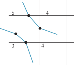
Figure 25.23: Knowing function values at grid points, we can estimate zero-crossings (black dots) by linear interpolation, and then connect the dots, in each cell, to estimate the level curve at level zero.
In doing so, however, we are ignoring additional data: At each estimated zero point, we can also make an estimate of the gradient of the function (see Figure 25.24) (or perhaps get the gradient directly as part of gathering the original data) and use these in estimating the shape of the level set.
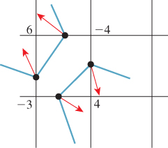
Figure 25.24: We can estimate gradients at the zero-crossings as well. Fitting a surface to the point-and-direction data gives a different estimate of the level-set.
This can be called an “Hermite” version (see Chapter 22) of marching squares. The extended marching cubes algorithm [KBSS01] uses this Hermite data to determine how the interior of a square appears: If the normals for the data in a square are similar, the algorithm defaults to standard marching squares. But if the point-normal pairs for a square (say (X1, n1) and (X2, n2)) are inconsistent (if n1 and n2 are not nearly parallel enough), then the square is treated differently: A new vertex, X, is placed in the square in such a way that it minimizes a quadratic error function,
as shown in Figure 25.25; in other words, X seeks to lie on the lines determined both by (X1, n1) and (X2, n2). (In 2D, this is trivial; in 3D, where there may be more contributing point-normal pairs, the minimization can be more complicated.) The newly inserted point is connected (with a pair of edges in 2D, or with a triangle fan based at X in 3D) to the zero-set on the boundary of the grid cell.
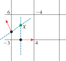
Figure 25.25: The normals at the two zero-crossings determine two lines, which intersect at a new point X.
There are two small problems.
1. If the normal vectors are sufficiently antiparallel, it’s possible that the minimizer X lies outside the square, and X must be adjusted to lie within it.
2. In the 3D case, if there are “extra points” X1 and X2 in two adjacent cells, we perform an edge flip on the contour edge that lies in the grid face between the two cells so that this edge now goes from X1 to X2.
![]() Argue that the “bad minimizer” problem above is the result of aliasing. What sampling is going on? Where are the too-high frequencies?
Argue that the “bad minimizer” problem above is the result of aliasing. What sampling is going on? Where are the too-high frequencies?
In estimating (at least in special cases) a surface point in the interior of a cell, the extended marching cubes algorithm suggests a different approach: If we had a surface point in adjacent cells, we could join these with edges (and faces, in 3D), using the points on grid edges as guides. Such an approach is called dual contouring. Ju et al. [JLSW02] developed a scheme for dual contouring of Hermite data, which involves two steps.
1. For each cell with differently signed vertices (i.e., not all positive or all negative), generate a mesh vertex within the cell by minimizing a quadratic error function.
2. For each edge with differently signed vertices, generate an edge (for 2D) or a quad (for 3D) connecting the minimizing vertices in the adjacent cells.
This algorithm has the pleasant characteristic that all cells are treated identically—there’s no threshold on when “normal vectors are close enough”—but there are subtleties: Again, the minimizing point for a quadratic error function may lie outside the cell, and furthermore, in areas where the surface is nearly planar the Hermite data for a cell may create a quadratic error function that is nearly degenerate (i.e., one whose zero-set is a whole line or plane) so that finding a minimizer is numerically unstable. Their work addresses this by careful numerical analysis, although their solution requires an ad hoc constant.
25.5.2. Mesh Repair
A mesh can be “broken” in all sorts of ways. Consider something as simple as a (hollow) triangle ABC in the plane. If we consider the edges as oriented as AB, BC, and CA, then the oriented boundary of the triangle, where the endpoint of each edge is counted as a +1 and the starting point as a −1, is empty. But if the edges are oriented as AB, BC, and AC, then the oriented boundary is 2C – 2A; if we were computing the boundary as a way to check whether the triangle was watertight, we’d find that it wasn’t. And if we used the oriented edges to compute normal vectors, the misoriented edge AC would cause problems with inside/outside determination. In a mesh whose representation contains an edge table, an algorithm closely related to the one for consistently orienting faces can be used to repair the edge table.
Often meshes created with rendering speed in mind have characteristics that generate problems, like T-junctions or nonwatertightness. Sometimes those created with the best intentions, like the Utah teapot, have problems. (The original teapot had no bottom!) So, while nice models are best to work with, we often encounter polygon soup—a collection of polygons that nearly form a nice surfacelike mesh—and we want to be able to make the most of what we’ve got. One example of this is in scanning, where a scanner may produce a great many points on a surface, and may even organize those points into triangles, but the triangles gathered from different views of the model may be inconsistent because of problems with registration of the views, or changing occlusion, etc. Such triangle soups need to be cleaned up to form consistent models for use in the rest of the graphics pipeline.
Ju [Ju04] has used his dual contouring for Hermite data to address this last problem. The ideas in the approach are simple, and the results are particularly attractive, so we sketch the method briefly here. The input is a collection of polygons; the output is a surface mesh that’s consistent, in some way, with the input polygons. Figure 25.26 shows the process (in 2D) in the case where the input mesh is already a closed polygon; in this case, the original mesh is reconstructed almost exactly, although it has been translated by an amount smaller than the grid cell.
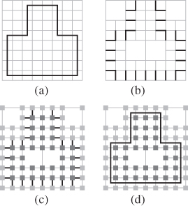
Figure 25.26: (Following [Ju04], Figure 3.) Ju’s model-repair method. (a) A model, embedded in a fine grid. (b) The grid edges that intersect the model, stored in an oct tree. Each cell touches an even number of such edges. (c) Signs at grid points (indicated by light or dark shading) generated from the set of intersection edges. (d) The model reconstructed by contouring the sign data.
The steps in the process are as follows.
1. The polygon soup is embedded in a uniformly spaced grid, and grid edges that intersect any polygon are marked as intersection edges. The cells containing such edges are stored in an oct tree. The choice of a fixed grid size implicitly represents a choice about aliasing: An empty polygon soup, and soup consisting of a single tetrahedron that fits entirely within one grid cell, will produce the same (empty) output. Thus, these two “signals” end up as aliases of each other.
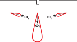
2. The intersection edges are used to generate signs at the grid points in such a way that each intersection edge exhibits a sign change. This may be impossible for certain inputs, as shown in Figure 25.27. These problems arise because of “boundary” in the input data.
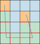
Figure 25.27: The U-shaped polygon soup generates several edges, but there’s no way to consistently assign signs to the grid cells so that each intersection edge exhibits a sign change. Cells with good labelings—most of the ones meeting the polyline—are in green. The problem arises at cells (in orange at the ends of the polyline) with an odd number of intersection edges.
Ju shows a method for “filling in” boundaries like this to create a set of intersection edges that can be given consistent signs. The filling-in approach generates fairly smooth completions of curves (2D) or surfaces (3D).
3. From the sign data (which can be extended to the entire grid), we can use marching cubes, or extended marching cubes or dual contouring, if we have normal data, to extract a consistent closed surface.
The method is not perfect. It can produce models in which the solids bounded by the output mesh have small holes (like those in Swiss cheese) or handles, and in areas where there are many bits of boundary in the original mesh the filling-in of the boundary may cause visually unattractive results. Nonetheless, the guaranteed topological consistency, and the high speed of the algorithm (due largely to the use of oct trees), make it an excellent starting point for any mesh-repair process.
25.5.3. Differential or Laplacian Coordinates
Just as derivatives are a central component of smooth signal processing and differences are critical in discrete signal processing, it’s natural to seek something similar in the case of mesh signal processing. If we have a signal s defined on the vertices of a mesh, the differences s(w) – s(v), where v and w are adjacent vertices, provide the analog to the differences s(t + 1) – s(t), t ![]() Z, for a discrete signal.
Z, for a discrete signal.
Second derivatives also arise in an important way: In Fourier analysis of a ![]() signal on an interval, we write signals as sums of sines and cosines, which are eigenfunctions of the second-derivative operator on the space of all signals. But considering second derivatives in a more concrete way, if we have a discrete signal
signal on an interval, we write signals as sums of sines and cosines, which are eigenfunctions of the second-derivative operator on the space of all signals. But considering second derivatives in a more concrete way, if we have a discrete signal
and we tell you s(0) and s′ (0), and s″ (t) for every t (using the “derivative” notion for what are really differences: s′ (t) denotes s(t + 1) – s(t), and s″ (t) denotes s(t + 1) – 2s(t)+ s(t − 1)), then you can reconstruct s(t) for every t: You use s′ (0) to reconstruct s(1), and use s″ (1), together with your knowledge of s(0) and s(1), to reconstruct s(2), and then continue onward.
Carry out the computation just described. Start with s(0) = 4, s′ (0) = 1, and s″ (1) = –1, s″ (2) = 0, s″ (3) = –1, and figure out s(1), s(2), s(3), and s(4).
Recording the value s(0) and derivative s′ (0), together with all the second-derivative values, thus provides an alternative representation of the signal. This representation has the advantage that if we want to add a constant to the signal, we can do so by only changing s(0) and leaving the rest of the data untouched.
Carry out the same computation as in the preceding exercise, but this time start with s(0) = 2; confirm that all other values shift by –2.
Similarly, we can add a linear variation to the signal (a steady increase or decrease in value) by changing just s′ (0). Thus, the second-derivative information captures the aspects of the signal that are unaffected by translation or shearing of the signal.
The analog, for meshes, is provided by the mesh Laplacians. Suppose that we have a mesh, and at each vertex we have a real number, which we’ll denote s(v) in analogy with the one-dimensional discrete-signal case. There’s no longer a notion of the previous or next signal value, but there is still a notion of adjacent values. Letting N(v) denote the 1-ring consisting of vertices adjacent to v, and |N (v) | denote the size of this set, we define the Laplacian of s at v to be
where the constant C is unimportant for now. We can bring the constant s(v) outside the sum, to get

where we’ve absorbed the number |N (v) | of neighbors of v into the constant C to make C′. In this form, we see the Laplacian expresses the difference between the signal value at the vertex v and the average of the signal values at the neighbors of v.
To be clear: The Laplacian is a function from “signals on the mesh” to “signals on the mesh.” Thus, if s is a signal, so is L(s), and L(s)(v) denotes the value of that signal at a particular vertex.
In analogy with the 1D situation, if you knew the value of s at some vertex v0 and at all but one of its neighbors, and you knew the Laplacian of s at every vertex, then you could compute the value of s at the last neighbor. And that might give you enough information to compute the value of s at another vertex, etc.
There’s a difference from the discrete-signal situation, however: The Laplacian values are not all independent.
Draw a tetrahedron, and write the numbers 1, 3, 0, and 5 at the four vertices, thus defining a “signal” s on the tetrahedron. Compute the Laplacian L(s)(v) at each of these vertices, using C = 1 as the constant. What do you notice about the sum of these values?
Thus, although the Laplacian of a signal once again represents the part that’s independent of the addition of a constant at every vertex, and some other kind of alteration similar to shearing in the 1D discrete-signal case, it’s no longer the case that an arbitrary set of values at vertices {h(v) : v ![]() V} can be treated as the Laplacian of some signal and “integrated” to recover the original signal. The usual solution is to ask for a signal s with the property that L(s)(v) – h(v) is as small as possible, typically by minimizing a sum of squares
V} can be treated as the Laplacian of some signal and “integrated” to recover the original signal. The usual solution is to ask for a signal s with the property that L(s)(v) – h(v) is as small as possible, typically by minimizing a sum of squares
Since the Laplacian is invariant under the addition of a constant to the signal, this minimization must typically be performed with one or more additional constraints, such as the value s(vi) at some small number k of selected vertices v1, ..., vk.
While we tend to have many functions defined on meshes—it’s common, for example, to evaluate some lighting model at each vertex of a mesh, and interpolate over edges and triangles—the function to which the Laplacian is most often applied is the one that returns, for each vertex, the coordinates of its location. For instance, we can regard the x-coordinate of each vertex as providing a signal value at that vertex. The same goes for the y- and z-coordinates. If we regard x : V ![]() R3 as the vector-valued function that takes each vertex to its xyz-coordinates, then it’s common to compute
R3 as the vector-valued function that takes each vertex to its xyz-coordinates, then it’s common to compute
These vectors, one per vertex, are sometimes called the Laplacian coordinates or differential coordinates for the mesh.
“Laplacian coordinates” is really a misnomer; a coordinate system should have the property that no two distinct points have the same coordinates (although in some cases, like polar “coordinates,” we allow a single point to be given multiple coordinates). But it’s easy to see that for a regular triangulation of a plane, the Laplacian coordinates at every vertex are zero, so any two planar parts of this mesh end up with the same “coordinates.” Perhaps “coordinate Laplacian” or “coordinate differentials” would be a better term, but “Laplacian coordinates” and “differential coordinates” are well established already.
Laplacian coordinates have a few obvious properties. First, they are invariant with respect to translation, that is, if M′ is a translated version of the mesh M, then the Laplacian coordinates at corresponding vertices are identical. Second, they are equivariant with respect to linear transformations, that is, if M′ is the mesh resulting from applying a linear transformation T to each vertex of M (e.g., rotating M 30° in the xy-plane), then the Laplacian coordinates at a vertex v′ in M′ can be computed from those at the corresponding vertex v by applying T. These facts, taken together, can be summarized by saying that Laplacian coordinates are equivariant with respect to affine transformations of meshes, as long as we remember that the action of an affine transformation on a vector ends up ignoring translations.
In summary: Laplacian coordinates on a mesh provide an affine-transformation-equivariant description of the geometry of the mesh. A mesh can be reconstructed from its Laplacian coordinates together with a small number of known mesh locations. And any vector-valued function of the vertices of a mesh can play the role of Laplacian coordinates if we reconstruct by solving a least-squares problem rather than seeking an exact solution.
25.5.4. An Application of Laplacian Coordinates
Nealen et al. [NISA06] describe an approach in which a mesh is “optimized” by adjusting vertex positions, but retaining the mesh connectivity. The technique is simple, and its good and bad features are self-evident.
The idea is to adjust the vertex locations to satisfy two goals: The first is that each vertex be as close to its original position as possible (with some vertices weighted more than others); the second is that the mesh Laplacian at a vertex, after adjustment, be as similar as possible to the nontangential part of the preadjustment mesh Laplacian. Since the mesh Laplacian represents the difference between a vertex and the average of its neighbors, this makes each vertex “want” to be the average of the neighbors, except for perhaps being displaced from the plane of the neighbors. (This description assumes that the neighbors actually lie more or less in a single plane, of course.)
Clearly the two goals—that vertices move toward their neighbor averages and that vertices not move at all—are in tension with each other. By adjusting the relative weights, we can arrange for greater shape preservation or greater mesh uniformity. Nealen et al. suggest some strategies for choosing weights that are widely effective.
In contrast to the usual vertex-and-face-table representation, we start with a mesh represented as a graph G = (V, E), with vertex set V and edge set E. We consider V as an n × 3 array whose ith row contains the x-, y-, and z-coordinates of the ith vertex, which we also store in a 3 × 1 column vector vi so that V = [v1, ..., vn]T.
We’ll compute the Laplacian coordinates, at vertex i by the rule
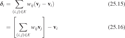
where for each i the weights wij sum to one, and may be chosen to be uniform, that is,
so that each edge arriving at vi gets equal weight, or by the cotangent rule, in which we set
where α and β are the internal angles of the vertices on either side of vj in the ring around vi (see Figure 25.28).1 We can then define
1. The rationale for the cotangent rule is presented in the web material for this chapter.
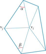
Figure 25.28: The vertex vi is surrounded by a ring of vertices, one of which is vj; the angles on either side of vj are called α and β. The cotangents of these angles are used in defining the weight of vj in the cotangent Laplacian vector at vi.
so that the sum ![]() is 1.
is 1.
If vi and its neighbors all lie in a plane, then the uniform Laplacian points from vi toward the average of the neighbor vertices, while the cotangent Laplacian is the zero vector. The two resultant Laplacians will be decorated with superscripts, as in ![]() , to indicate their nature.
, to indicate their nature.
Our goal is to find new vertex positions ![]() (i = 1, ..., n) that are both (a) near the old positions, and (b) arranged so that their Laplacians are similar, in some way, to the old Laplacians. The first condition can be expressed by writing
(i = 1, ..., n) that are both (a) near the old positions, and (b) arranged so that their Laplacians are similar, in some way, to the old Laplacians. The first condition can be expressed by writing
where Wp is a diagonal matrix of weights, which gives us control over which position constraints are most important to us. Clearly this system can be solved by letting V′ = V, but we’ll be adding further constraints in a moment.
Since there are n vertex positions vi, each in 3-space, the matrix V is n×3. What size is each of the other matrices in Equation 25.20?
The second condition, on the Laplacian, can be written in the form
where again we’ve included a diagonal weighting matrix WL, and where L is the matrix of some Laplacian coordinate transform (i.e., the first row of LV is the Laplacian at vertex v1, etc.). The matrix F is a target for the Laplacians. Taken together, in block matrix form, we’ll be solving
Nealen et al. observe that if we set L = Lu and F contains the cotangent Laplacian coordinates of all vertices, the resultant mesh preserves the details of the original but the shapes of individual triangles are improved. If we set W to the identity, all vertices are allowed to move equally and the triangle shapes are slightly improved. If, on the other hand, we set the weight for a vertex to be proportional to the mean curvature at that vertex, then vertices at highly curved points will remain fixed, while others move. The problem with this is that often there are a few vertices with very high curvatures, and so if we map curvatures to weights linearly, only a few vertices get at all constrained. Nealen et al. suggest an alternative: They compute
the fraction of all vertices whose curvatures are no more than κ, and assign to each vertex of curvature κ a weight proportional to C(κ). The weights are stored in a matrix WL. The constant of proportionality is a tuning parameter.
The result is a system that manages to improve triangle shape while maintaining the mesh features at high-curvature points.
On the other hand, if we set L = Lu and F = 0, then we actually smooth the mesh, removing some amount of noise from the shape. Nealen et al. discuss other variants of this approach.
We have not discussed how to set the positional weights, Wp. Can you think of any points in a typical object (e.g., a video-game character) for which large weights might be appropriate?
In both the triangle shape optimization and mesh smoothing methods, we need to solve the system of equations in Equation 25.22. This consists of a 2n×n matrix multiplied by an unknown n × 3 matrix to get a 2n × 3 matrix. We can solve this problem for one column of unknowns at a time. That is we can solve
by solving
where Xi indicates the ith column of X, for i = 1, 2, 3. To solve, we can compute an LU decomposition of A [Pre95]. Fortunately, this single decomposition can then be used to find each column of X.
25.6. Mesh Applications 2: Deformation Transfer and Triangle-Order Optimization
We conclude this chapter with two more advanced applications related to meshes. The first is deformation transfer, in which two meshes of objects with some relationship (e.g., two quadrupeds) are matched at a few key points, after which any deformation of the first mesh can be automatically transferred to the other. The second is an approach for restructuring a mesh’s face table so that during rendering the mesh will tend to use a GPU most efficiently.
25.6.1. Deformation Transfer
Suppose that using a motion-capture system, we have captured the varying position of a human actor over time; in other words, we have a mesh M (the source mesh) with a fixed connectivity (i.e., a fixed set of triangles, represented as vertex-index triples), and a sequence Vi, (i = 0, 1, ...) of positions for the vertices of the mesh (i.e., V0 is the set of vertex positions at time 0, perhaps representing the actor standing upright at rest, V1 is the set of vertex positions at time 1, etc.). We’d like to transfer this motion sequence to a different mesh (the target)—a video-game character, for instance—but one that may not have a realistic human form. Or perhaps we have a recorded sequence of positions for a horse, but we want to apply them to a camel, which was unavailable for motion capture. We can consider the difference between V0 and Vk as a deformation of the known model; our desire is then to transfer this deformation to the target mesh M′, with a possibly different set of triangles and vertex locations W0, to get a new set of vertex locations Wk. We’ll follow the approach of Sumner and Popovi![]() [SP04] (see Figure 25.29).
[SP04] (see Figure 25.29).
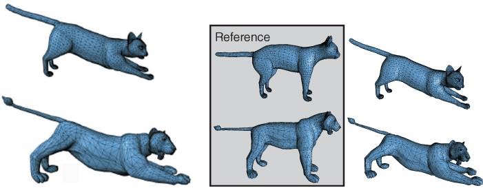
Figure 25.29: We start with a source and a target mesh, shown at left, a triangle-by-triangle correspondence between them (in this case, the correspondence is the fairly obvious one), and a deformation of the source mesh, shown at the top right. The deformation transfer algorithm provides a transformation of the target mesh that’s analogous to the deformation of the source mesh. (Courtesy of Robert Sumner and Jovan Popovi![]() .)
.)
Because we are considering only deformations, we need only look at k = 1 and apply the same technique to each subsequent value of k. So we can relabel things a bit for simplicity: We’ll use Vi to indicate the initial position of vertex i in the source mesh (i.e., its position in V0), and ![]() to indicate its deformed position (i.e., its position in V1). For notational simplicity, it’s helpful if everything we consider is a vector rather than a point. We therefore pick an “origin” OM for M, and express each vertex as an offset from this origin:
to indicate its deformed position (i.e., its position in V1). For notational simplicity, it’s helpful if everything we consider is a vector rather than a point. We therefore pick an “origin” OM for M, and express each vertex as an offset from this origin:
We do the same for ![]() , that is,
, that is,
and similarly for M′, although we’ll choose the origin OM′ independently. (It’s a good idea to use something like the center of mass of M as the origin for M, and similarly for M′, to avoid roundoff errors in later numerical computations.)
We’ll similarly use wi and ![]() for the (vector) position of the ith target vertex before and after deformation. We’ll assume that we’re given vi,
for the (vector) position of the ith target vertex before and after deformation. We’ll assume that we’re given vi, ![]() , and wi for all i, and we wish to find
, and wi for all i, and we wish to find ![]() for all i.
for all i.
To make the connection between the deformations of the source mesh M and the target mesh M′, we need a correspondence, C, between them. This is provided, in the Sumner-Popovi![]() formulation, by a collection of pairs C = {(si, ti)
formulation, by a collection of pairs C = {(si, ti) ![]() Z × Z : i = 1, 2, ..., c} between triangles. A pair (si, ti) indicates that the target triangle with index ti should deform similarly to the source triangle with index si. The set C is a relation on triangle indices: It may specify that triangle 7 in M′ is to deform similarly to both triangles 2 and 96 in M (in which case the pairs (2, 7) and (96, 7) would both be in C), or that triangles 11 and 12 in M′ should both deform like triangle 4 in M, in which case C would contain both (4, 11) and (4, 12). It’s not required that every triangle index of M appear as the first element of some pair in C, nor that every index of M′ appear as the second element of a pair. Nonetheless, it may be easiest to imagine C as being nearly a one-to-one correspondence, in which a triangle on the horse’s head corresponds to a triangle on the camel’s head and a triangle on the horse’s left front foot corresponds to a triangle on the camel’s left front foot, etc. The problem of building or describing such a correspondence in the first place is a separate one; it’s possible to try to algorithmically guess correspondences between parts, etc., but it’s probably easiest to have a user indicate correspondences between a few dozen key points, and then use some kind of breadth-first-search-followed-by-relaxation approach to “grow” the correspondence outward from these key points.
Z × Z : i = 1, 2, ..., c} between triangles. A pair (si, ti) indicates that the target triangle with index ti should deform similarly to the source triangle with index si. The set C is a relation on triangle indices: It may specify that triangle 7 in M′ is to deform similarly to both triangles 2 and 96 in M (in which case the pairs (2, 7) and (96, 7) would both be in C), or that triangles 11 and 12 in M′ should both deform like triangle 4 in M, in which case C would contain both (4, 11) and (4, 12). It’s not required that every triangle index of M appear as the first element of some pair in C, nor that every index of M′ appear as the second element of a pair. Nonetheless, it may be easiest to imagine C as being nearly a one-to-one correspondence, in which a triangle on the horse’s head corresponds to a triangle on the camel’s head and a triangle on the horse’s left front foot corresponds to a triangle on the camel’s left front foot, etc. The problem of building or describing such a correspondence in the first place is a separate one; it’s possible to try to algorithmically guess correspondences between parts, etc., but it’s probably easiest to have a user indicate correspondences between a few dozen key points, and then use some kind of breadth-first-search-followed-by-relaxation approach to “grow” the correspondence outward from these key points.
We’ll now set about describing deformation transfer as an optimization problem. Before we write the optimization, however, we need one more enhancement of the meshes.
Suppose we have a triangle with vertices v1, v2, and v3, which are to be sent to another triangle with vertices ![]() 1,
1, ![]() 2, and
2, and ![]() 3. It’s natural to think of the transformation from one to the other in terms of the affine transformations we use all the time in graphics: some sort of translation, and an associated linear transformation. The problem is that the two triangles each lie in a plane, and there are infinitely many affine transformations taking one triangle (and its plane) to the other (and its plane): The off-plane part of the transformation is completely unconstrained.
3. It’s natural to think of the transformation from one to the other in terms of the affine transformations we use all the time in graphics: some sort of translation, and an associated linear transformation. The problem is that the two triangles each lie in a plane, and there are infinitely many affine transformations taking one triangle (and its plane) to the other (and its plane): The off-plane part of the transformation is completely unconstrained.
Examine a 2D analog: Find an affine transformation T from R2 to R2 that takes the line segment from (0, 0) to (1, 0) on the x-axis into the line segment from (0, 1) to (0, 2) on the y-axis. Now compose your transformation with the transformation S : R2 ![]() R2 : (x, y)
R2 : (x, y) ![]() (x + 3y, y), that is, form R = T Ο S, and show that R transforms the segments exactly the same way that T did.
(x + 3y, y), that is, form R = T Ο S, and show that R transforms the segments exactly the same way that T did.
We therefore add a new vertex v4 that’s offset one unit along the normal to the triangle defined by v1, v2, and v3,
and a corresponding new vertex to M′. Now there’s a unique affine transformation taking v1, ..., v4 to ![]() 1, ...,
1, ..., ![]() 4. Writing the transformation as a combination of a translation with a linear map, we see that the linear map Q must send the vectors Vi – V1 to
4. Writing the transformation as a combination of a translation with a linear map, we see that the linear map Q must send the vectors Vi – V1 to ![]() for i = 2, 3, 4. Writing
for i = 2, 3, 4. Writing
we have ![]() ; we can thus compute the translation d as
; we can thus compute the translation d as
where O is the origin of 3-space.
Notice that we have added one new vertex to the original and deformed meshes for each triangle. So our starting point becomes
• An original mesh M, with an enlarged vertex set that we’ll still denote with the same symbols, {vi}, and with each “triangle” associated to four vertices
• A deformed mesh ![]() , with a corresponding enlarged vertex set
, with a corresponding enlarged vertex set
• A second mesh, M′, with an enlarged vertex set {wi}
• A correspondence C between triangles of M and M′
• For each triangle t of M, an affine transformation v ![]() Stv + dt that transforms the four vertices of t to the four vertices of t in
Stv + dt that transforms the four vertices of t to the four vertices of t in ![]()
It’s convenient to think of the triangle t in M as represented by its index in M’s triangle table so that St and dt are indexed by integers.
Our goal is to find a collection of transformations of the target mesh M′ that are “as much like” those of M as possible; writing the target transformation for a target triangle s in the form
our goal is to have Ts and St be as similar as possible whenever (t, s) ![]() C. Notice that we’ve ignored the translations of the source mesh here, and concentrated on the intrinsic deformation and translation of each triangle. Because we’ve ignored the source translations, our solution will not be unique: We can add any constant translation to all the
C. Notice that we’ve ignored the translations of the source mesh here, and concentrated on the intrinsic deformation and translation of each triangle. Because we’ve ignored the source translations, our solution will not be unique: We can add any constant translation to all the ![]() vectors and get an equally good solution. By explicitly setting the displacement
vectors and get an equally good solution. By explicitly setting the displacement ![]() for one triangle s in the target, we remove this ambiguity.
for one triangle s in the target, we remove this ambiguity.
There is a further problem: If the vertex wi is shared by two triangles s1 and s2, it’s possible that
In that case, the vertex will be sent to two different places by the two different transformations, and thus will not define a transformation on the mesh, M′, but rather on the set of triangles in the mesh. Letting N (wi) denote the set of all triangles that contain the vertex wi, we therefore seek transformations satisfying
We express this goal numerically as the problem of minimizing
subject to
where ||A||2 denotes the sum of the squares of the entries in the matrix A. (The square root of this quantity is called the Frobenius norm of the matrix A.) This is a quadratic optimization problem, which can be solved by standard numerical techniques. (As an aside, we caution you against writing your own quadratic optimizer, unless you are an expert in numerical analysis. Instead, find one you like, and get to be an expert in using it.) One problem with this formulation is the number of constraints: There’s a constraint for every pair of triangles that meet at a vertex. Even if every vertex had degree three, this would still be a number of constraints that’s equal to the number of vertices, which is very large in general. The problem begs for reformulation.
Sumner and Popovi![]() perform a natural transformation: Instead of treating the transformations Ti as unknowns, with constraints on where they send the mesh vertices, they treat the eventual vertex locations
perform a natural transformation: Instead of treating the transformations Ti as unknowns, with constraints on where they send the mesh vertices, they treat the eventual vertex locations ![]() as unknowns, and write the transformations Ti in terms of these.
as unknowns, and write the transformations Ti in terms of these.
Recall that each source deformation transformation S was given by an expression of the form ![]() . If we knew the final positions
. If we knew the final positions ![]() of the target vertices, then the target deformations would similarly be given by expressions of the form
of the target vertices, then the target deformations would similarly be given by expressions of the form ![]() . The entries of the matrix T are evidently linear functions of the unknown positions
. The entries of the matrix T are evidently linear functions of the unknown positions ![]() . The minimization problem becomes
. The minimization problem becomes
where the Ssj are all known, and in the expression for T,
the factor W–1 is known as well. Only ![]() is unknown. Thus, the summation above is a huge quadratic in the unknown positions. If we place all of these unknown positions into a 3n × 1 vector x, then the minimization can be rewritten in the form
is unknown. Thus, the summation above is a huge quadratic in the unknown positions. If we place all of these unknown positions into a 3n × 1 vector x, then the minimization can be rewritten in the form
where A is a large, sparse matrix. In fact, if we place the x-coordinates of all the unknowns in the first n entries of x, and then the y-components in the next n, and then the z-components in the third n entries, the matrix A ends up block-diagonal, consisting of three n × n blocks.
To minimize such a quadratic expression, we set the gradient to zero and solve; the result is the system of linear equations
The matrix A depends only on the known data, so it needs to be computed only once, as does Q = ATA. And solving a problem of the form
can be done with the LU decomposition of Q (which we need only compute once) and back-substitution. The LU decomposition can be found blockwise for the three blocks, further simplifying the computation.
The trickiest part of implementing this algorithm concerns bookkeeping: Transforming from an optimization in the form of Equation 25.35 to an optimization in the form of Equation 25.37 involves careful index manipulation. If you actually want to implement this idea, we strongly suggest that you first do so in two dimensions, and that you work with an example mesh consisting of no more than about five vertices and seven edges (which play the role of triangles in the two-dimensional formulation). It will also help to formulate the computations in a language like Matlab or Octave, in which matrix formulations are built into the language. Once you have made that work, transferring to some other language is much easier, especially since you can use the matrix-formulated implementation as a reference during debugging.
25.6.2. Triangle Reordering for Hardware Efficiency
As you know, the graphics pipeline, as implemented in the GPU, has several stages. Any one of these can be a bottleneck. For some models, transforming vertices dominates, and modern GPUs tend to cache such transformed vertices because of this. When it comes to generating triangles to be drawn, we get better cache use if those that share vertices are processed at nearly the same time. Triangle strips are one way to produce this kind of mesh locality. For other models, there may be enormous complexity that is mostly hidden (e.g., a model of an office building may contain millions of triangles, of which only a few hundred are visible from any particular office space). In these cases, if we can draw the visible triangles first, then a z-test will tell us that the fragments generated by other triangles are not visible, and thus that the lighting and shading computations for those fragments need not be performed. Of course, backface culling also will help reduce the rendering load by about 50% on average. By clever clustering of triangles, it’s possible to address the cache-miss problem quite effectively. The obvious solution to the “overdraw” problem, however, is view-dependent: If we can sort the triangles front to back, we can minimize overdraw. But such a sort order will likely break up the clusters that addressed the vertex-cache problem. Nonetheless, this front-to-back approach provides the core of the algorithm. We can find a front-to-back order for the triangles by creating a graph whose nodes are triangles and where there’s a directed edge from t1 to t2 if t1 obscures (partly or completely) t2. Performing a topological sort on this graph gives a drawing order, assuming that the graph is acyclic. We’ll return to the problem of cycles presently.
Nehab et al. [NBS06] have developed a solution that incorporates the best of both approaches, in the presence of backface culling: They create clusters that are large enough that only a small amount of cache-missing is introduced (compared to the optimal), but which also substantially reduce overdraw when the clusters are drawn in a particular order. Their approach relies on three key ideas.
1. If two polygons’ normal vectors have a dot product of –1, then their sort order will have no impact on overdraw, because whenever one is front-facing, the other will be back-facing, and hence culled. For dot products greater than –1, the chance of overdraw increases with increasing dot product.
2. If their normal vectors have a positive dot product, it’s possible that one obscures the other from many viewpoints, but the other never obscures the first. In this case, any sort order where the obscuring polygon comes before the obscured reduces overdraw.
3. The preceding observations are still true even for planar clusters of polygons, and even if the clusters are nearly planar rather than planar.
Figure 25.30 shows these situations. Notice that if the mesh is convex, then any sort order will minimize overdraw, because for a convex mesh, there’s never any overdraw at all. Even for the nonconvex wave-shaped rooftop mesh of Figure 25.31, it’s still possible to draw the polygons in an order that creates no over-draw. With these examples in mind, the algorithm has two broad steps: First, we create nearly planar connected clusters of triangles using a k-means-like clustering algorithm [HA79]; then we determine a sort order for the clusters by creating a graph whose nodes are the clusters and in which there’s a directed edge from c1 to c2 if c1 obscures c2 more than c2 obscures c1 (averaged over all possible points of view). The edges are given weights depending on how much more c2 obscures c1 than c1 obscures c2. We then attempt a topological sort on this graph, using edge weights to break any cycles that arise.
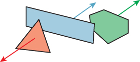
Figure 25.30: The sort order of the blue and red polygons is immaterial because of back-face culling; the blue polygon obscures the green from some viewpoints, but the green never obscures the blue.

Figure 25.31: Drawing the rooftop regions of the building in increasing numerical order, and using backface culling, will prevent overdraw no matter what the viewpoint.
25.6.2.1. Clustering
The user must provide a number, k, of clusters to compute; k provides a tradeoff between vertex-cache efficiency and overdraw efficiency. (The authors report that between 10 and 100 clusters suffice for models on the order of 100,000 triangles.) We then select k random triangles and grow clusters from them. In general, a k-means algorithm has two steps that are alternated: adding items to a cluster based on a “distance” to some representative for the cluster, and updating the representative. For clustering points in a plane, the representative is typically the centroid of the cluster, the distance is Euclidean, and at each iteration, each item is added to the cluster whose center, from the last iteration, is nearest.
In the version of k-means used in this algorithm, the clusters begin with k randomly chosen “seed” triangles. Each cluster is represented by a centroid and a cluster normal; initially these are the centroid and face normal for the starting triangle. The clusters are “grown” by a breadth-first search (based on triangle adjacency) from the seed triangles, which are assigned a distance of zero from the cluster center. A triangle f adjacent to a triangle g of cluster C is assigned a distance equal to that of g plus 1 – nf · nC + ![]() , where nf and nC are the face normal and average cluster normal, respectively, and is a small constant that ensures that triangles topologically close to the seed are preferred over those that are far away. Once distances from each face to all cluster centroids have been thus computed, each face is assigned to the cluster of the nearest centroid. In the second step, the cluster centroid and the average cluster normal nC are recomputed, and the iteration is restarted. Because of the dot-product term in the incremental distance function, triangles closely aligned with the cluster normal tend to fall into the cluster, while those tilted away do not; this results in cluster boundaries tending to be aligned with sharp creases in the mesh. Note that a triangle may be adjacent to a cluster C along two of its edges (or all three); in this case, we add the incremental distance to the lowest of the already-computed distances of the neighbors.
, where nf and nC are the face normal and average cluster normal, respectively, and is a small constant that ensures that triangles topologically close to the seed are preferred over those that are far away. Once distances from each face to all cluster centroids have been thus computed, each face is assigned to the cluster of the nearest centroid. In the second step, the cluster centroid and the average cluster normal nC are recomputed, and the iteration is restarted. Because of the dot-product term in the incremental distance function, triangles closely aligned with the cluster normal tend to fall into the cluster, while those tilted away do not; this results in cluster boundaries tending to be aligned with sharp creases in the mesh. Note that a triangle may be adjacent to a cluster C along two of its edges (or all three); in this case, we add the incremental distance to the lowest of the already-computed distances of the neighbors.
25.6.2.2. Sorting
Once we have computed the clusters, we compute a value I(c1, c2) that says how much cluster c1 obscures cluster c2, from enough viewpoints that our computation is a good estimate of the average occlusion, and we use this to build a graph whose nodes are labeled by the clusters. The value I is computed in pixels: It’s meant to represent the number of possible overdraws that result from drawing c2 before c1, on average. If I(c1, c2) > I(c2, c1), we should draw c1 before c2, so we place a directed edge from c1 to c2 in the graph, with edge weight I(c1, c2) – I(c2, c1), which is always positive.
If the resultant graph admits a topological sort (which ignores the weights), we’ll use it. If not, we want a sort order that minimizes the weights of all “violations” (i.e., cases where c2 comes before c1 in the sort order, even though there’s an edge from c1 to c2). Unfortunately, this problem is NP-complete [Kar72], but a simple greedy heuristic works well. It’s based on an algorithm for topological sort in which we choose as a starting node any vertex with only outgoing edges, and as an ending node any vertex with only incoming edges; we then remove these vertices and their associated edges from the graph and find a topological sort for the remainder.
In an unsortable graph, the approach above fails when every node is part of some cycle (i.e., has both incoming and outgoing edges). In this situation, we remove the node at which the weight sum for incoming edges is most different from the weight sum for outgoing edges, placing it on the “winning” side of the ordering (i.e., making it the next cluster to be drawn), and then continue with the normal topological sort.
Finally, within each cluster, we sort the triangles in a way to optimize mesh locality (i.e., to avoid vertex-cache misses), using some triangle-stripping algorithm like that of Hoppe [Hop99].
The results are impressive, generating up to 40% savings on overdraw for a model with 150,000 triangles. Of course, it’s possible to construct exotic meshes for which almost no planar patch clusters exist; the algorithm will perform badly on these. But for the kinds of meshes encountered in everyday games, for instance, the algorithm works well.
Sander et al. [SNB07] have improved on this algorithm, and we anticipate further research in this area, in which geometry and efficient computations are combined.
25.7. Discussion and Further Reading
The geometric study of meshes is a growing field, known as discrete differential geometry. Because of its close relationship to smooth differential geometry, you should start by becoming familiar with that material. A particularly gentle introduction is O’Neill’s book [O’N06]; Millman and Parker’s book [MP77] is a good follow-up. For discrete differential geometry, there are tutorials available [MDSB03], and at least one textbook [BS08].
The situation in what we’ve called “mesh flattening” (and what has come to be known as “parameterization of meshes”) is not as hopeless as our remarks might suggest. There does not seem to be any single ideal approach to parameterization yet, but there’s been substantial progress beyond the simplest approaches [SPR06, CPS11, SSP08].
The structure of a mesh and the structure of the underlying graph are closely related. The graph Laplacian has been used to address problems like graph partitioning and clustering; analogs have been used in mesh partitioning.
Ray-mesh intersection testing, since it’s in the critical path for ray tracing, has been much studied. And because of its relevance to animation, so has collision detection for meshes. Many ideas can be shared between the two topics. Haines and Moller [AMHH08] give a complete overview, with details on many algorithms.
Mesh optimization has been widely studied, along with the relationship of mesh “smoothing” operations to digital filter design [Tau95] and to mean curvature flow [DMSB99, HPP05]. Methods that allow small connectivity alterations were popularized in graphics by Witkin and Welch [WW94], and can frequently be useful in adjusting meshes where some vertex degrees are so large or small that it’s impossible to have all adjacent triangles approximately equilateral.
Despite all the research on meshes, they may, in fact, turn out to not be the ultimate shape representation model for graphics. For rendering, the discontinuity of reflection (you can adjust an incoming ray an arbitrarily small amount and get an arbitrarily large change in the reflected ray) is a serious problem, especially when one is trying to prove claims about convergence. The way that surfaces “condense” geometric information (like curvature) to low-dimensional subsets (vertices and edges) is reminiscent of the abstraction of the point light source, which condenses the light emitted from a small area into light emitted from a single point. Such an abstraction is convenient for some simple forms of rendering, but in fact makes others considerably more difficult. It’s possible that mesh representations of surfaces will someday be regarded only as limiting cases for some other preferred kind of representation in which geometry generically has at least C2 continuity.
Nonetheless, meshes are an active area of research. Pick up any SIGGRAPH proceedings from 2000 to 2012 and you’ll find at least a dozen papers that concentrate on meshes in some form, and we anticipate that this trend will continue for some time. Read such papers once with an open mind, to get ideas, and again with a menagerie of wild meshes, like the non-locally-flat example of Figure 25.14, and the highly wrinkled example of Figure 34.11, and a mesh built from an array of pieces shaped like Figure 25.32, where no two adjacent normal vectors are similar, and see whether the claims hold up. Another good test case is two large spheres that have been joined by removing a small triangle from each and either gluing the edges together directly, or splicing in a small triangular-prism-shaped “corridor” between them. (The boundary of the 2-ring of a vertex of that prism may well not be connected, for instance!)
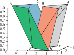
25.8. Exercises
Exercise 25.1: Our algorithm for computing the boundary of a triangle mesh involved iterating through all the faces, and it runs in O(f) time. Describe a connected triangle mesh with O(f) boundary edges, thus showing that the O(f) runtime is as good as possible.
Exercise 25.2: If we have a one-dimensional path mesh (i.e., each vertex has one or two edges meeting it), we can place it in the plane by assigning random locations to the vertices. In general, the result will not be an embedding: Edges will tend to cross one another. In 3-space, however, there’s plenty of room, and with high probability the use of randomly assigned locations will result in an embedded path mesh. In this exercise, you’ll show that for any surface mesh, there’s an embedding in some Euclidean space. The idea is simple: For an n-vertex mesh, we’ll place the mesh in Rn by placing vertex 1 at location (1, 0, ...), vertex 2 at location (0, 1, ...), etc. We then place edges and faces in the obvious way, using linear interpolation.
(a) Explain why the embeddings of triangles (i, j, k) and (i′, j′, k′) do not intersect unless the sets S1 = {i, j, k} and S2 = {i′, j′, k′} have nonempty intersection. (b) Show that if S1 ![]() S2 contains a single index p, then the associated embedded triangles intersect only at vertex p.
S2 contains a single index p, then the associated embedded triangles intersect only at vertex p.
(c) Show that if S1 ![]() S2 = {p, q}, then the associated embedded triangles intersect in the embedded edge associated to {p, q}.
S2 = {p, q}, then the associated embedded triangles intersect in the embedded edge associated to {p, q}.
Exercise 25.3: Consider the mesh shown in Figure 25.32. By replicating it to the left and right, and then replicating the resultant strip in the front and back directions, we get a mesh in which no more than two adjacent triangles have remotely similar normal vectors. Show that such a mesh is likely to be a worst-case challenge to the polygon ordering algorithm of Nehab et al., as described in Section 25.6.2.
Exercise 25.4: (a) We sketched an algorithm for computing the boundary of a surface mesh by hashing edges. Adapt this to detect all contours of a mesh, where a contour edge is one where the normals to the two adjacent faces have dot products, with a view vector v, of opposite signs, and the contour is the set of all contour edges. (b) Contour edges can be generally formed into loops, although as we said, two loops may share one or more vertices. Design an O(E) algorithm for assembling the E contour edges into loops. Hint: Use hashing again.
Exercise 25.5: The paper by Nealen et al. [NISA06] suggests using the mean curvature to compute weights. Make an argument for using the absolute value of the mean curvature instead. Can you think of any argument against this, or any rationale for why it might be an unimportant improvement, even if it works?