
Chapter 24. Implicit Representations of Shape
24.1. Introduction
We introduced implicit functions in Chapters 7 and 14 as a means for defining shapes. Implicitly defined shapes, like the circle defined by x2 + y2 = 1, or the sphere defined by x2+y2+z2 = 1, or far more general shapes defined by equations of the form F(P) = c for some complicated function F, serve several roles in graphics. First, for a wide class of functions, computing ray-surface intersections with such shapes is fairly easy. Second, it’s sometimes convenient to represent surfaces like “the boundary between water and air” in a simulation implicitly, because it’s very easy to change the topology of an implicitly defined surface (by changing either F or c), while it’s generally difficult to do so for parametrically defined surfaces. Third, in many applications we find ourselves with data defined on a grid of points (the temperature at each point in a nuclear reactor, for instance, or the material density at each point in a CAT scan of a brain) and we wish to visualize this data; often, seeing the level surface (the set of points where the function has a particular value) for a function that’s consistent with the observed data can help us understand the data. In this chapter, we introduce implicit curves and surfaces and discuss how they are used to model shapes, how they can be used in ray tracing and animation, and how they can be converted to polyhedral meshes.
The main advantages of implicit representations are the general smoothness of the shapes defined this way, the simplicity of creating quite general shapes, the ease of defining shapes whose topology changes over time, and the ability to exactly compute surface normals and other geometric properties (many of which are difficult to estimate for polyhedral surfaces). The disadvantages are that converting an implicit representation to a polygon mesh suitable for most renderers can be very expensive, and that the ability of implicits to represent multiple topologies can also make it difficult to control the topology of an implicitly defined shape.
24.2. Implicit Curves
In Chapter 7 we discussed two ways to describe a line in the plane: either parametrically (writing P + td, for values t ![]() R) or implicitly (in a form like Ax + By + C = 0, with A and B not both zero; or in vector form, (X – P) · n = 0, where n is a nonzero vector in the plane and P is a point of the line—the set of points X satisfying this equation forms a line containing P and perpendicular to n). In addition, we observed that it was particularly easy to find the intersection of a parametric line with an implicit line. Similarly, in 3-space we could define a plane implicitly, and ray-plane intersections were easiest when the ray was parametric and the plane implicit.
R) or implicitly (in a form like Ax + By + C = 0, with A and B not both zero; or in vector form, (X – P) · n = 0, where n is a nonzero vector in the plane and P is a point of the line—the set of points X satisfying this equation forms a line containing P and perpendicular to n). In addition, we observed that it was particularly easy to find the intersection of a parametric line with an implicit line. Similarly, in 3-space we could define a plane implicitly, and ray-plane intersections were easiest when the ray was parametric and the plane implicit.
We further generalized to talk about implicitly defined curves in the plane that were more general than lines, like the circle, defined by x2 + y2 = 1, or more general curves (see Figure 24.1). More generally, if we have any function z = F(x, y) defined on the plane,1 such as the height of the terrain at each location (x, y) in some hilly area, then the sets of points defined by F(x, y) = c are called contour lines and are an example of a level set of a function (in the sense that they are the points at the same level on the graph of F). Level sets are sometimes also called isocurves of F. Mathematics books often discuss level sets by only considering the case c = 0; that’s because the level set where F(x, y) = c is the level set where G(x, y) = 0 if we define the function G by
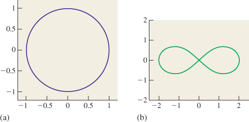
Figure 24.1: Two implicit curves in the plane. (a) The circle is defined by x2 + y2 = 1, or by x2 + y2 – 1 = 0. (b) The lemniscate of Bernoulli is defined by (x2 + y2)2 = 2c(x2 – y2); changing c adjusts the angle at which the lines cross at the center of the figure eight.
1. We are following the mathematics convention that the xy-plane is horizontal and that the z-direction is vertical, because the xy-plane is of primary interest to us for the time being; were we to follow the graphics convention, we’d have to describe a circle by an equation like x2 + z2 = 1 instead of x2 + y2 = 1; the familiarity of the xy-formulation seems worth the inconsistency in the choice of axes.
Thus, you’ll sometimes encounter the term zero set rather than “level set.”
Because the points of the curve are defined indirectly—we simply have the function F which tells us whether a point is on the curve or not—we also say that the curve is an implicit curve. If the formula for F is sufficiently complicated, it may not even be clear whether the set defined by F(x, y) = c is empty or not.
In the cases we’ve discussed so far—the line, circle, and lemniscate—the first two implicit curves are very smooth, but the third has a self-crossing. The distinction among them is the nature of the functions defining them. In general, if C is the level set F(x, y) = c, then C consists of disjoint simple closed curves if at every point P of C, the gradient ![]() F(P) is nonzero.
F(P) is nonzero.
In the case of the line, the function FL(x, y) = Ax + By + C has gradient ![]() , which is nonzero everywhere. For the circle, the function FC(x, y) = x2 + y2 has gradient
, which is nonzero everywhere. For the circle, the function FC(x, y) = x2 + y2 has gradient ![]() , which is zero only at (x, y) = (0, 0), which is not a point of the circle. But for the lemniscate,2 where
, which is zero only at (x, y) = (0, 0), which is not a point of the circle. But for the lemniscate,2 where
2. The subscript “B” is for Bernoulli.
we have
which, at (x, y) = (0, 0), is the zero vector. At places where the gradient is zero, an implicit curve can have singularities (self-intersections, sharp corners, tangencies). This is not, however, an if-and-only-if condition. For instance, the circle can also be defined by the equation
which has gradient zero at every point of the circle. In short, a nonzero gradient ensures that the curve is nice, but the curve’s niceness tells us nothing about the gradient.
The preceding example also shows that the function that defines an implicit curve is by no means unique: Many functions can define the same curve. That’s another drawback of implicits.
How common are zeroes in the gradient? A back-of-the-envelope argument says they’re fairly common. If we set the first term of the gradient to zero, we’ve got one equation in two variables (which defines a curve in the plane); if we set the second to zero as well (defining a second curve in the plane), we’ve got two equations in two variables. If they were linear equations, we’d generally have a solution; because they may be nonlinear, we can merely say that we might well expect to find isolated solutions to the two equations (i.e., points where the two curves intersect). If we chose a level c at random, we would not expect F(x, y) = c to hit any of these gradient zeroes, but if we were to vary c, we might well expect that for certain values of c, the level set for c contains a gradient zero. This can be thought of in terms of a physical analogy, as shown in Figure 24.2: If we take our function to be the height of the terrain above or below sea level, then when the sea level is c, the level set for c is the shoreline. As the tide rises, c changes, and the shape of the shoreline changes. For example, two adjacent islands may be separated by water at high tide (so that the level set consists of two closed curves—the shorelines of each island); as the tide drops, the islands may become joined by an isthmus so that at low tide, the shoreline is one long curve. For some value of c, the level set changes from two curves to one curve; at the point where the curves join, the gradient is zero.
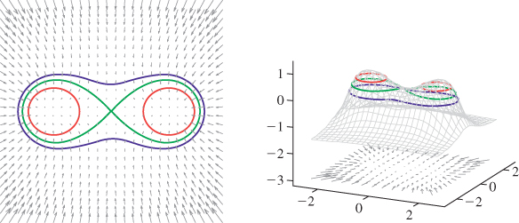
Figure 24.2: A topographical map and side view of two islands. At high tide (two almost-circular red curves) the islands are separated and the shoreline has two parts; at low tide (large blue curve) the islands are joined by an isthmus, and the shoreline is a single curve. At mid-tide (green figure-eight curve), the shoreline has a singular point, where the gradient of the height function is zero. In both figures, the faint gray arrows are scaled versions of the gradient of the implicit function.
The gradient of an implicit curve, when nonzero, has another important function: It always points in the direction of the normal vector to the curve. (This, and the claim that when the gradient is nonzero the curve is smooth, are consequences of the implicit function theorem [Spi65].) We can see this in the case of the unit circle: At the point (x, y), the gradient is ![]() , which is indeed parallel to the normal, which is
, which is indeed parallel to the normal, which is ![]() .
.
We can also see the kinds of problems that arise when the gradient is zero by looking at the function F(x, y) = 1 + x3 – y2, shown in Figure 24.3 and the level
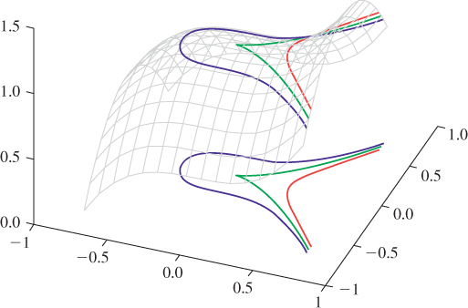
Figure 24.3: The graph of F(x, y) = 1 + x3 – y2 and its associated level curves for c = . 95, 1, and 1. 05. The level curve for c = 1 has a cusp at the origin, where the gradient is zero. This example shows that the topology of the level set need not change at a place where the gradient is zero.
set defined by F(x, y) = 1: At the point (x, y) = (0, 0), the level set has a sharp cusp, even though nearby level sets are completely smooth.
24.3. Implicit Surfaces
The notions of the preceding section all generalize to three dimensions quite simply: If we have a function w = F(x, y, z) defined on 3-space (e.g., the temperature at each point in a room), we can find the set of points
at which F takes on the value c; in general, this is a smooth surface in 3-space. As a concrete example, if F is the function defined by
then the level set for c = 1 is the unit sphere in 3-space, as shown in Figure 24.4. (In three dimensions, level sets are sometimes called isosurfaces or level surfaces.)
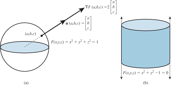
Figure 24.4: (a) The sphere is defined as the zero set of the implicit function F(x, y, z) = x2 + y2 + z2 – 1; at a typical point P = (x, y, z) of the sphere, the gradient is parallel to the ray from the origin to P, hence parallel to the normal vector to the sphere at P. (b) The cylinder can be defined implicitly by x2 + y2 = 1.
Just as in the two-dimensional case, if P = (x, y, z) is a point of some level surface, then the gradient ![]() F(x, y, z) is parallel to the normal vector to the surface at P. And if the gradient is nonzero everywhere, then the surface is actually smooth. On the other hand, if the gradient is zero at some point of a level surface, there may be a self-intersection there, or a corner of the surface, or a sharp point.
F(x, y, z) is parallel to the normal vector to the surface at P. And if the gradient is nonzero everywhere, then the surface is actually smooth. On the other hand, if the gradient is zero at some point of a level surface, there may be a self-intersection there, or a corner of the surface, or a sharp point.
Again, as in the curve case, a randomly chosen level surface of a smooth function F is unlikely to contain any gradient zeroes, but if we continuously vary the level (or the function F), we should expect to encounter some gradient zeroes.
Finally, the intersection of a ray defined by a point P and a direction d with an implicit surface defined by F = c can be computed by solving F(P + td) = c (see Figure 24.5).
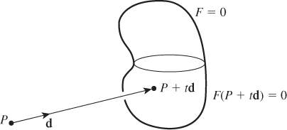
Figure 24.5: The intersection of a ray (defined by a point P and a direction d) and an implicit surface defined by F(x, y, z) = c must occur at a point Q = P + td (for some value of t) which satisfies F(Q) = 0. So to find the intersection, we can solve F(P + td) = c for the unknown t; the intersection point is then P + td.
For instance, if F(x, y, z) = x2 + y2 + z2, and we consider the intersection of the ray with P = (–2, 0, 0) and d = (1, 1/3, 0) with the level set F = 1 (the unit sphere), we must solve
that is,
Applying the formula for F, this gives
which is a quadratic in t, namely,
whose solutions are
these correspond to the points
on the sphere.
The intersections we just computed depended on the coordinates (Px, Py, Pz) of P and the coordinates (dx, dy, dz) of d. Express the intersection points in terms of these coordinates rather than their particular values, and determine under what conditions an intersection exists.
With these generalities on implicit curves and surfaces in mind, we can now move on to discuss the ways in which implicit functions are most often represented.
24.4. Representing Implicit Functions
While the examples in the preceding section were given in terms of explicit polynomial formulas, such an approach becomes impractical when we want to use implicit surfaces for modeling particular shapes: What polynomial in three variables, for instance, has a level set that has the shape of a dolphin? It’s clear that searching for the appropriate degree and coefficients is an intractable task.
Instead, an implicit function is often represented by samples, the values of the function on a fixed grid of points such as the integer points of the plane or 3-space. (Such a representation arose naturally from the gathering of regularly spaced data in scientific experiments or surveying). Of course, knowing a function’s values at integer points does not tell us the values at noninteger points. Indeed, between any pair of integer points, a function can take on any values at all. It’s conventional to assume that the samples are so closely spaced that between samples, the function “doesn’t do anything funny” so that, for instance, one might assume that between samples, the function takes on values that are determined by simple combinations of the values at the sample points (the same way we took values at points of a polygon mesh in Chapter 9 and extended them to define a function on the entire mesh). If we consider the plane, for instance, as a polygon mesh (with each polygon being a square), with values known at the vertices, we could interpolate over the interiors of squares. The methods of Chapter 9 don’t help us, because they assumed that the mesh was made of triangles.
24.4.1. Interpolation Schemes
There are several approaches to extending a function defined on the integer grid in the plane to a function defined on the whole plane.
24.4.1.1. Conversion to Triangles
A first approach is to convert the mesh of squares into a mesh of triangles, as shown in Figure 24.6(a), by adding a diagonal to each square. Because there are two choices for the diagonal (and there’s no particular a priori reason for the choices to be the same for every square), this approach seems unsatisfactory, although for finely sampled data it’s often quite adequate. Alternatively, as Figure 24.7(b) shows, we can break each square into four triangles by adding a point at the center. We typically assign this center point a value that’s the average of the four corner values; we can then interpolate using the method of Chapter 9.
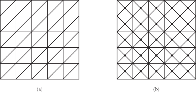
Figure 24.6: (a) The mesh of squares defined by the integer points of the plane can be converted to a mesh of triangles by drawing a diagonal in each square. (b) It can also be done in a more symmetric way by adding a vertex at the center of each square (shown as a small dot) and breaking the square into four triangles.
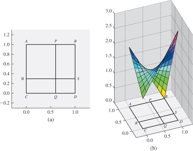
Figure 24.7: (a) If we know the values vA, vB, vC, and vD of a function at the points A = (0, 0), B = (1, 0), C = (0, 1), and D = (1, 1), we can compute a value at the point (x, y) inside the unit square by first interpolating values linearly at the points P and Q of AB and CD, respectively, and then interpolating between these; alternatively, we could interpolate the values at the points R and S of the edges AC and BD, and then interpolate between those. In either case, the resultant value is (1 – x)(1 – y)vA + x(1 – y)vB + (1 – x)yvC + xyvD. (b) The graph of the resultant function when vA = 1, vB = 3, vC = 2, and vD = 0. Notice that constant-x and constant-y cross sections of the graph are linear.
24.4.1.2. Bilinear Interpolation
A different approach is to insist that the interpolation, along each edge of the square, should be linear. With this in mind, we can take a square in our grid, as shown in Figure 24.7, and determine the value at the point (x, y) in the square by linear interpolation along a pair of parallel edges to get the values vP = (1–x)vA+ xvB at P and vQ = (1 – x)vC + xvD at Q, and then interpolate linearly between these to get (1 – y)vP + yvQ as the value at the interior point (x, y) of the unit square. (For any other square, we must use the fractional parts of the coordinates of x and y in place of x and y).
Writing this out in terms of the four corner values, we get
as the value at the point (x, y) of the unit square. Because the blending functions are all bilinear in x and y, this is called bilinear interpolation.
24.4.2. Splines
Bilinear interpolation can be seen as a blending of values at the four corners by certain polynomials, suggesting that any interpolating spline would also work, and indeed this is true: If we take any function h that’s 0 everywhere except in the range –1 ≤ x, y ≤ 1, where it’s nonnegative, and is 1 at (0, 0), we can define a function
that takes on the known values v(i, j) at each integer point (i, j). If, in addition, the function h has the property that F is everywhere 1 when all the v(i, j) values are 1, then in general the value F(x, y) will lie between the minimum and maximum values known at the four corner points. Examples of such functions are
• The box function on the unit square – ![]() < x, y <
< x, y < ![]()
• The bilinear basis function
If we weaken the requirement that h(0, 0) = 1, other functions like the bicubic B-spline basis function can also be used.
Even more general functions can be chosen to play the role of h, but the key idea is simple: h represents how the effect of the value at each vertex fades as we move away from that vertex. In doing so, h encodes something of our belief about the implicit function that we’re representing by samples.
24.4.3. Mathematical Models and Sampled Implicit Representations
As the previous sections show, given samples of a function on the integer grid, there’s no single answer to the question, “What function do these samples come from?” And without an answer to that question, there’s no hope of answering, “What implicit curve (or surface) do these samples define?” In the case of data gathered in an experiment, there may be little knowledge on which to base our choice of function, but it’s clear that if the variation of the function over a grid cell is so large that the values at the corners of the grid cell fail to represent this variation faithfully, any interpolation and level-set finding is bound to give a wrong answer. It’s therefore common to assume that the function being sampled is band-limited (i.e., its Fourier transform contains no frequencies higher than some specified frequency ω), and that the samples are spaced close enough to ensure that we can accurately reconstruct any such function from its samples. Indeed, if the samples are spaced twice as close as needed for reconstruction, then simple linear interpolation serves to approximate the function quite well, as we saw in Chapter 18. Unfortunately, approximating the true function F0 by a function F whose value at each point is very near the value of F0 does not ensure that a level set of F resembles the corresponding level set of F0. To understand this, consider a very gradually sloping beach. A very small change in tide level can create a drastic shift in the shoreline; alternatively, a beach shaped only slightly differently can have a drastically different-looking shoreline. Thus, the level sets of F and F0 need not be very similar at all.
This apparent contradiction—the defining functions are similar, but the implicit curves or surfaces are different—can be resolved, in part, by scaling: If we insist that we consider only functions F and level sets F = c with the property that the gradient, at each point of the level set, has magnitude at least 1, then an alteration of F by some small enough amount δ results in a motion of the level surface that’s O(δ). For acquired data, guaranteeing this property of the gradient may be infeasible. For cases where we are building implicit functions ourselves, it may be feasible. But if our interest in implicits is in their ability to represent changing topologies as the level value changes, then at the topology-changing level, we must have a point where the gradient is zero (so the assumption that the magnitude is greater than one is violated). In short, although it’s possible to make guarantees of correctness for certain classes of implicit functions, in practice the hypotheses may be unenforceable or impractical.
24.5. Other Representations of Implicit Functions
Implicit surfaces are sometimes referred to as “blobbies,” because it’s so easy, with functions like F(x, y, z) = x2 + y2 + z2, to create small blobs. Indeed, radially symmetric functions, translated to various points and summed, allow one to create multiple blobs. If z = f(r) is a rapidly decreasing function of r with f(0) = 1, then we can define
which will be a function with maxima at or near the points Pi (assuming that they’re far enough apart), and the level set at level c = 0.9, for instance, will consist of approximately spherical blobs around the Pi. If two of the points Pi are very close, then their associated blobs will merge into a single larger blob, and this idea is the basis for modeling shapes with implicit functions: By choosing the points Pi carefully, we can build up a shape as a sum of blobs. This approach to modeling has been very thoroughly investigated [BW90, WGG99]; Bloomenthal’s book [BW97b] provides a great many details. One approach, in which blobs blend in a very predictable way, was developed by Wyvill et al. [WMW86]. Critical to its success is finding a function f with the property that when blobs merge, the volume of the resultant blob is approximately the sum of the individual volumes.
If we consider an implicit function F as not defining a surface where F = 0, but rather a volume (the points P where F(P) ≥ 0), then there are further operations we can consider. For instance, if F and G both define shapes, then max(F, G) defines the union of the shapes (the max is positive only if one of the two functions is positive), while min(F, G) defines the intersection. Unfortunately, the function max(F, G) is not necessarily smooth, even if F and G are. Since smoothness is often important in guaranteeing the quality of results for implicit surfaces, these functions are sometimes replaced by smooth approximations; with these smooth approximations, we get approximations of the union and intersection of shapes. By starting from simple shapes, defined by individual functions, and combining them with operations like translation, rotation, smooth-max, smooth-min, etc., we can create implicit representations of quite complex shapes (Figure 24.8 shows an example). Wyvill [BEG98] describes this blob tree approach in detail.
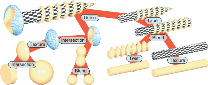
Figure 24.8: A complex shape created from simple implicit surfaces combined in a “blob tree,” which defines a complex implicit function in terms of unary and binary operations on simpler implicits (Courtesy of Erwin de Groot and Brian Wyvill.)
Another approach to describing implicit functions, based on so-called “radial basis functions,” is described in the web materials for this chapter.
24.6. Conversion to Polyhedral Meshes
An implicit function represented by samples on a grid can be converted to a polyhedral mesh; we’ll discuss marching cubes, the most widely known method of doing so. Other implicit-function representations can be converted indirectly, first by sampling on a grid and then by applying marching cubes, but there are cases where it’s possible to quickly find a point on each component of an implicit surface, and from this seed point construct the surface component directly [WMW86]. A rough estimate suggests that in an n × n × n grid, one expects O(n2) polygons in an implicit surface mesh, but since marching cubes examine every cube of the grid, it takes Ω(n3) time; thus, in cases where the structure of the implicit function gives a priori information, it can be very useful in reducing the isosurface-extraction time.
We’ll first examine the iso-set extraction problem in two dimensions; most of the complexity of the problem is present there, but the pictures are easier to understand than those in three dimensions.
Our starting point is a grid of values; the desired output is a set of polylines representing the zero-set of the function associated to the values. We’ll refer to this set of polylines as the output “mesh,” in preparation for the three-dimensional example, even though it consists of only vertices and edges. Constructing the mesh can be divided into two tasks: determining the topology of the mesh (how many vertices and edges, and which are connected to which) and the geometry of the mesh (determined by the actual locations of the vertices). Figure 24.9 shows this process.
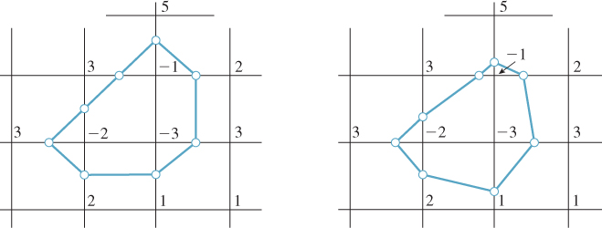
Figure 24.9: Starting from a grid of values, we first determine the topology of the isocurve for an associated function. Vertices are indicated by small circles at midpoints of edges. We then adjust the locations of the vertices to better match the input values (i.e., the small circles move to the place where a linear function on the edge would have a zero crossing). Thus, the process of isocurve extraction is divided into topological and geometric tasks.
To simplify matters, we’ll assume that no vertex has value 0; we’ll return to this simplification after developing the remainder of the algorithm.
We’ll also assume that if the topology of the isocurve within some grid square is indeterminate, then any answer consistent with the data is satisfactory. (We’ll also return to this simplification later.)
Finally, we’ll assume that the function defined by values at the four vertices has no maxima or minima in the interior of each square, and interpolates the values linearly on each edge of the grid.
With these assumptions, we can classify each grid point as a “+” or “−” point, depending on whether the value there is positive or negative. If the ends of an edge have opposite signs, then the function must pass through zero somewhere on the edge, so we will place a vertex on that edge. Up to symmetries, there are only a few possibilities, shown in Figure 24.10. For each possibility, we’ve shown a way to draw in the isocurve within the grid square in a way that’s consistent with the edge crossings on the boundary. In case (c), there are multiple ways to connect the edge crossings. We’ve shown two that result in isocurves with no self-intersections.
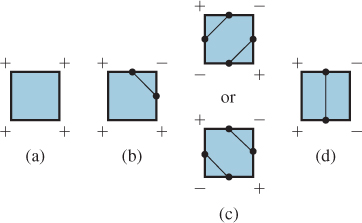
Figure 24.10: Patterns of signs on a grid square. (a) All plusses (or minuses). (b) One plus (or one minus). (c) Two diagonally opposite plusses. (d) Two adjacent plusses. All other cases are rotations or reflections of these. In each case, we’ve marked a dot at the center of each edge through which the isosurface passes, and shown possible patterns of edges by which these can be connected.
Choosing one way to fill in each possible configuration of edge crossings, we produce a topologically valid isocurve configuration.
Having done so, we can move each isocurve vertex from an edge midpoint to the correct location on the edge (i.e., where a linear function on the edge would have a zero crossing).
This isosurface construction approach has some rather nice properties.
• We can give each isocurve vertex a name consisting of the x- and y-coordinates of the endpoints of the segment it lies on, with the leftmost or lower vertex coming first, so a vertex on the segment from (1, 2) to (1, 3) would have a name (1, 2, 1, 3).
• We can process the grid of squares one at a time. For each square, we do the following.
– Find the isocurve vertex associated to it.
– If the vertex is new (we can use a hash table with the name as an index to check this in O(1) time), we assign a new index to the vertex name, and add this index to our vertex table; if it’s old, we do nothing with it.
– For each new vertex, we use the values at the ends of the associated edge to determine its exact location, and record this in the vertex table.
– Examine the pattern of plusses and minuses to figure out what edges must be added (we can do this with a lookup table in which the four plusses and minuses serve as a 4-bit binary index); then we add these edges to the edge table.
• The resultant set of isocurves has the property that every vertex (except those on the very boundary of the grid) is shared by exactly two edges; hence the resultant isocurves are all simple closed curves or polylines.
The square-at-a-time property will extend to 3D as well; because that 3D algorithm is called “marching cubes,” this 2D algorithm can be called marching squares. In practice, it may make sense to process a whole row of squares at once to favor cache coherency.
Let us now return to the assumptions made at the start of our discussion of marching squares.
We assumed that no grid vertex had the value 0. If a vertex has value 0, but none of its neighbors do, we can adjust the value slightly (to, say, .001 times the next smallest vertex value adjacent to it). We then proceed with the rest of the algorithm, but at the very end, we adjust the positions of isocurve vertices that lie on edges leaving this grid vertex so that they are all this single vertex. This means that up to four different isocurve vertices may be at the same location so that the isocurve no longer necessarily consists of disjoint simple closed curves and polylines. Often, however, just two vertices get moved to sit at the grid vertex, and the edge between them ends up with zero length (see Figure 24.11), while the closed-curves-and-arcs property continues to hold. If four vertices all collapse to a single grid vertex, the property no longer holds.
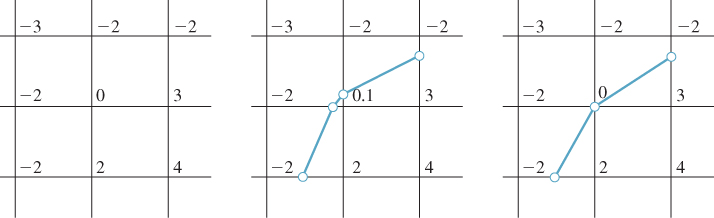
Figure 24.11: One grid vertex has value 0; we adjust the value slightly and compute the isocurve (which passes near the grid vertex), and then, at the end, we move the two nearby vertices to the grid vertex so that the edge between them shrinks to nothing.
If two or more adjacent vertices have value 0, more complex problems arise. For instance, if all four vertices of a grid square have value 0, then all edges of the square should be included in the isocurve, as perhaps should the whole square itself, which would make the isocurve no longer be a curve! We address these cases in the same way as the previous case: We adjust all 0 values slightly, compute the isocurve, and then adjust vertices at the end. But if a vertex lies on a grid edge where both ends have value 0, rather than moving the vertex to one end or the other, we place it at the middle of the edge. The result of this is an isocurve that’s topologically correct in any grid cell with no 0 values at its corners, and is topologically consistent even in cells where there are zeroes. This is an instance of our second assumption—that in indeterminate cases, any consistent answer is acceptable—except that we do not always include the entire grid edge between two zeroes.
The difficulties of handling zeroes in the data are intrinsic to the original problem: In places where the graph of a function is nearly horizontal, level curves are unstable, in the sense that a small change in the input (the data values) results in a large change in the resultant level curve.
24.6.1. Marching Cubes
The marching cubes algorithm for finding an isosurface of a function specified at grid vertices in 3-space is exactly analogous, although there are some subtleties. Once again, it’s easiest to assume that all input values are nonzero; if there’s a zero in the input, perturb it by a small random amount, compute the isosurface, and then move the isosurface vertices back to the proper locations as we did in the marching squares algorithm.
Again, the output associated to a particular cube in the grid is determined by the pattern of plusses and minuses at its vertices. Since there are eight vertices, each with a plus or minus sign, we can encode the pattern of plusses and minuses with an 8-bit binary number; this can be used to index into a table of presolved examples, containing the vertex and triangle table for the mesh structure of the output; the actual locations of the vertices in the vertex table are once again determined by interpolation along edges of the grid.
Figure 24.12 shows two of these cases: The first generates a single triangle as output, and the second generates a rectangle, which would generally be represented by two triangles.
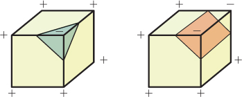
Figure 24.12: Two examples of patterns of plusses and minuses, and the associated bits of iso-surface.
In the marching squares algorithm, a grid edge contained either no isocurve vertex or one isocurve vertex. In the latter case, each of the two adjacent grid squares had an edge that ended at that vertex, so each vertex met two edges, and the edges therefore fell into long chains (which either were closed curves, or terminated at the boundary of the grid). In the marching cubes algorithm, adjacent cubes meet along a face, as shown in Figure 24.13; these faces share isosurface vertices, but the way that the isosurface vertices are connected by edges within each copy of the face might not be consistent. If this happens, the resultant model of the isosurface will have edges in the interior of the grid, which is inappropriate. It’s critical therefore that the 256 models used for the 256 possible cases in the marching cubes algorithm be pairwise consistent so that the resultant isosurface mesh either is closed or has boundary edges only on the boundary of the input grid.
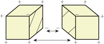
Figure 24.13: Two adjacent cubes in the marching cubes algorithm share a single face. The same four vertices appear on the four edges of this face, but the edges that join together pairs of isosurface vertices in each cube are not consistent with one another; the surface that results will have a boundary rather than being a closed surface.
As in the marching squares algorithm, the marching cubes algorithm is very well suited for a one-plane-of-data-at-a-time approach, in which the output associated to a plane of grid cubes is computed all at once, and then the next plane of grid cubes is loaded into memory.
24.7. Conversion from Polyhedral Meshes to Implicits
Implicit representations have some important advantages over polyhedral models, as we’ve mentioned. It’s not only possible to convert from implicit representations to polyhedral ones, but it’s also possible to do the opposite: Given a nice enough polyhedral mesh, we can find a function F whose level set resembles the mesh. One class of meshes that is “nice enough” are ones with the property that the complement of the mesh—the set of all points in 3-space not on the mesh—can be divided into two sets with the property that each mesh face is on the boundary of both sets. If the mesh is a pair of cubes, for instance, one of the sets would be the interiors of both cubes, and the other would be the region exterior to both. Every face of the cube has the interior on one side and the exterior on the other. By contrast, a Möbius band is not “nice enough,” because its complement consists of a single connected set.
When a mesh has this “two set” property we can declare one set to be “positive” and the other set “negative,” and then define a function F on 3-space by the rule that F(P) is the minimum straight-line distance from P to the mesh, multiplied by –1 if P is in the “negative” region. This is an implicit function (known as the signed distance transform of the mesh) whose zero-set is the mesh. Unfortunately, if we represent this function by grid samples, the level-zero isosurface will not be exactly the original mesh in general, but it will be very similar to it, provided the grid samples are closely enough spaced.
In general, however, interconverting between implicit and polyhedral models tends to be lossy, and should probably be avoided.
24.8. Texturing Implicit Models
Because implicitly defined models are generally not equipped with texture coordinates, it’s common to use volume textures to texture them. Such volume textures can be procedurally defined, by a rule like
which varies between dark brown and light brown cylindrical rings; an implicit object textured with such a function gets a (very simple) wood-like appearance. (Textures like this one, which can be expressed as a function of two coordinates, are sometimes called projection textures, because one can imagine the texture being projected from a 2D image out into space [Pea85].) More often, however, textures for implicitly defined objects are defined explicitly via a volumetric representation such as a voxel grid with colors at each voxel.
To avoid the cost of creating and storing all the voxels, while only a few are used for texturing, one can also use a hierarchical data structure like an oct tree in which most cells are empty, but ones near the implicit surface are filled in. This is also a natural structure to use in a painting interface, in which an artist directly paints texture (color, normals, displacement) onto a surface: In broad constant areas, unrefined structure represents the texture compactly; in areas with finer detail, we can refine the oct tree so that it can hold this detail. This idea has been developed in some detail by DeBry et al. [DGPR02] and Benson and Davis [BD02].
24.8.1. Modeling Transformations and Textures
Just as we typically describe a polyhedral model in some modeling space, and then apply various transformations to it so as to put it in a particular location and orientation in world space, we typically define implicit models in some modeling space as well, and transform them into world space. For example, we define a sphere by the equation F(x, y, z) = x2 + y2 + z2 − 1 = 0; to translate this sphere to the point (1, 3, 4) we replace F by
Setting G(x, y, z) = 0 then gives a unit sphere centered at (1, 3, 4). We can consider G as being constructed from F by the rule
where T is the transformation “translate by (−1, −3, −4),” that is, exactly the inverse of the transformation we wanted to apply to the sphere.
The implicit formula for an ellipsoid of radii (2, 1, 1) in x, y, and z is x2/4 + y2 + z2 – 1 = 0.
(a) Letting F(x, y, z) = x2 + y2 + z2 – 1, is the implicit equation of our ellipsoid F(x/2, y, z) = 0 or F(2x, y, z) = 0?
(b) What simple scaling transformation takes points of the unit sphere to points of our ellipsoid?
(c) How are parts (a) and (b) related?
In general, if S is a surface defined implicitly by the function F (i.e., if F(s) = 0 if and only if s ![]() S), the surface T(S) = {T(s) : s
S), the surface T(S) = {T(s) : s ![]() S}, where T is an invertible linear transformation, is implicitly defined by the function
S}, where T is an invertible linear transformation, is implicitly defined by the function
In fact, the transformation T need not be linear—it need only have an inverse. This means that transformations like
which rotates each z = c slice of 3-space by a different amount so that the strip [–1, 1] × 0 × R gets twisted into a helical shape, can be used to apply a helical deformation to any implicitly defined object.
A shape that’s been modeled implicitly and then transformed can be textured in world space (the texture at a point P with F(T–1(P)) = 0 is determined by the coordinates of P itself) or in modeling space (the texture is determined by the coordinates of T–1(P)).
24.9. Ray Tracing Implicit Surfaces
When we wanted to compute the intersection of a ray (parameterized in the usual form t ![]() P + td) with an implicitly defined sphere, we ended up solving a quadratic equation in t which arose by writing out F(P+td) = 0, where F was the implicit function defining the sphere. But if the implicit object is more general, it’s possible that the equation F(P + td) = 0 might have an enormously complicated form, and there may be no simple formula for finding its roots. In this case, we must fall back on numerical techniques for root finding [Pre95].
P + td) with an implicitly defined sphere, we ended up solving a quadratic equation in t which arose by writing out F(P+td) = 0, where F was the implicit function defining the sphere. But if the implicit object is more general, it’s possible that the equation F(P + td) = 0 might have an enormously complicated form, and there may be no simple formula for finding its roots. In this case, we must fall back on numerical techniques for root finding [Pre95].
As we mentioned in Section 24.8.1, if S is an implicit surface defined by a function F, and T is a linear transformation, then the surface T(S) is defined by F° T–1. As hinted at in Exercises 7.17 and 11.13, the problem of intersecting a ray t ![]() P + td with T(S) can be recast as the problem of intersecting a different ray with S. Since T(S) is defined by F ° T–1, a point of our ray is on T(S) exactly when
P + td with T(S) can be recast as the problem of intersecting a different ray with S. Since T(S) is defined by F ° T–1, a point of our ray is on T(S) exactly when
That’s the same equation we get when asking when a point of the ray t ![]() T–1(P) + tT–1(d) is on the surface S. Finding a ray-surface intersection in the untransformed version of the implicit surface may be straightforward (as we’ve seen with the plane and the sphere in earlier chapters). This means that if you’re willing to model a scene by applying transformations to several implicitly defined shapes like spheres or cylinders, you can ray-trace the scene by taking each ray, and for each object, apply the inverse of the object’s modeling transformation to the ray’s basepoint and direction vector. You then intersect this “back-transformed” ray with the pretransformed object to find an intersection point Q and a normal vector n to the object. Applying the modeling transformation to Q and its normal transformation to n gives the intersection point and normal in world space.
T–1(P) + tT–1(d) is on the surface S. Finding a ray-surface intersection in the untransformed version of the implicit surface may be straightforward (as we’ve seen with the plane and the sphere in earlier chapters). This means that if you’re willing to model a scene by applying transformations to several implicitly defined shapes like spheres or cylinders, you can ray-trace the scene by taking each ray, and for each object, apply the inverse of the object’s modeling transformation to the ray’s basepoint and direction vector. You then intersect this “back-transformed” ray with the pretransformed object to find an intersection point Q and a normal vector n to the object. Applying the modeling transformation to Q and its normal transformation to n gives the intersection point and normal in world space.
For scenes of modest complexity, this works well. For highly complex scenes, it’s a better idea to use a bounding-box hierarchy to first determine which transformed implicit shapes the ray has a chance of intersecting, and then do the intersection test only on those that pass this test.
24.10. Implicit Shapes in Animation
![]() Implicit curves or surfaces can also be used in animation; within physically based animation, they play a major role under the name level set methods [OS88]. In such methods, there’s some initial object of interest that is defined either by an implicit equality (F0(x, y, z) = 0) for surfaces or by an inequality (F0(x, y, z) ≥ 0) for solids.3 Various forces act on the surface or solid attempting to deform it in some way; these, in turn, are treated as attempts to deform the defining function F0. One ends up with a differential equation of the form
Implicit curves or surfaces can also be used in animation; within physically based animation, they play a major role under the name level set methods [OS88]. In such methods, there’s some initial object of interest that is defined either by an implicit equality (F0(x, y, z) = 0) for surfaces or by an inequality (F0(x, y, z) ≥ 0) for solids.3 Various forces act on the surface or solid attempting to deform it in some way; these, in turn, are treated as attempts to deform the defining function F0. One ends up with a differential equation of the form
3. These methods can also be applied in two dimensions to implicit curves.
where the vector field (x, y, z) ![]() v(x, y, z) describes how the level set of the function Ft should move at the point (x, y, z). (The field v can be time-varying as well.) Solving this differential equation for Ft as a function of t gives the evolving shape of the object as the forces act on it.
v(x, y, z) describes how the level set of the function Ft should move at the point (x, y, z). (The field v can be time-varying as well.) Solving this differential equation for Ft as a function of t gives the evolving shape of the object as the forces act on it.
Typically the forces act on the implicit surface itself, and therefore they may be known only at points where Ft = 0. On the other hand, the values of the function F at points far from those where F = 0 are unimportant, and so it’s possible to keep track of Ft only near locations where Ft = 0. One way to do this is to extend Ft to nearby points by signed distance [LKHW03]; another way is to keep track of the values of Ft only in a narrow band around the set Ft = 0, and extend the field v to that band [AS95]. In either case, the function Ft is usually represented by voxel samples.
The advantage of the level-set approach to animation is that changing topology (like droplets of water merging into a single larger drop) is easy to generate. The method has been used to produce many of the most realistic fluid animations to date [EMF02] (see Figure 24.14).
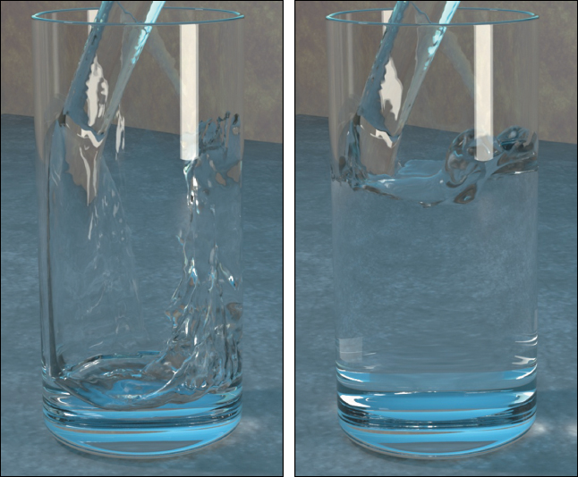
Figure 24.14: Water animated by the level-set method. Notice how droplets form and merge. (Courtesy of Stephen Marschner, ©2002 ACM, Inc. Reprinted by permission.)
24.11. Discussion and Further Reading
There’s a duality between implicit and parametric models that we mentioned in Chapter 7, making them suited for different applications, and with the peculiar characteristic that finding the intersection between two models is easier when one is parametric and the other is implicit.
Implicit representations of shape as an artistic tool have fallen out of favor somewhat in recent years, but they have grown in popularity as shape representations for simulation. This may be related to GPUs, where polygonal representations are strongly supported, or it may be related to the fact that having an artist build a function on all of space to get a surface that occupies just a tiny part of it is somewhat awkward. This awkwardness is partly avoidable by using the signed distance from the shape (positive outside, negative inside). To be useful in an implicit definition, this signed distance function need only be represented close to the zero-set: Its values far away cannot matter. The same is true for the volumetric texture functions described earlier in the chapter. Perhaps methods like this will rejuvenate the use of implicitly defined models.
One charm of implicit surfaces is that their geometry (i.e., tangent planes, curvature, etc.) is completely determined by the defining implicit function, and can be computed analytically. The web material for this chapter describes the computation of curve and surface curvature, for instance.
24.12. Exercises
Exercise 24.1: Explain why the formula of Equation 24.14 gives a function with the property that for any point (x, y) where x and y are both nonintegers, the value F(x, y) lies between the minimum and maximum values of v at the corners of the square containing (x, y) if h has the property that when all the v(i, j) are 1, the function F is everywhere 1.
Exercise 24.2: In the marching squares algorithm, we chose one of two possible ways to connect vertices in the case where the signs at the corner of a grid square alternated; the choice we made was independent of the values at the four corners.
(a) Explain why, if we drew a diagonal from the northeast to the southwest corner of each grid square, and treated the resultant collection of triangles as a mesh with values at vertices, the piecewise-linear interpolation of those values has a graph whose level-zero slice is consistent with our choice.
(b) Explain why, if we’d chosen the alternate diagonal for each grid square, it would be equivalent to making the other choice.
(c) Devise an algorithm in which we add a new vertex to the center of each grid square, with edges from this vertex to the four corners, and we assign a value to the new vertex that’s the average of the four corner values. Use this new mesh (and these new values) to generate an isocurve for the piecewise linearly interpolated function. (Your new isocurve will have vertices both on the original grid edges and on the new edges you added from each center vertex to the corners. (d) Explain how this revised approach can lead to either of the two possible ways of connecting the edge vertices in the + – + – case.