
Chapter 29. Light Transport
29.1. Introduction
In this chapter we develop the rendering equation, which characterizes the light transport in a scene. We do this first for a scene in which there is no transmissive scattering, only reflection, and then generalize to handle transmission as well. In all but the simplest cases, the rendering equation is impossible to solve exactly. Approximation methods are therefore essential tools. The dominant approximation method involves estimating certain integrals by so-called Monte Carlo integration, that is, randomized integration algorithms, which we discuss in the next chapter. To assist with understanding the convergence properties of such algorithms, we can consider various kinds of light transport, some of which are amenable to study with one technique, some with another. For instance, a sequence of mirror reflections that conveys light from a point source to the eye must be treated rather differently from a sequence of diffuse reflections of illumination from an area light source. In fact, the phenomena produced by various kinds of light-transport paths can also be quite different at a perceptual level; we discuss this briefly, as well.
29.2. Light Transport
With the notion of the radiance field in hand, and that of the bidirectional reflectance distribution function (BRDF), we can now discuss light transport in general. We begin with the case of a scene consisting of empty space and purely reflective objects (i.e., there is nothing that’s partly transparent, and light reflects from the surfaces of objects—there’s no subsurface scattering to consider). The scattering of light from an object is therefore described by the BRDF, which we’ll denote fr (the “r” standing for “reflection”). This special case conveys the main ideas but avoids some complexities. Having developed this first situation, we’ll generalize to other kinds of scattering, but with very few important changes.
We’ll continue with the assumptions of Chapter 26, that the scattering of light by a material comes in two parts: mirror and Snell-transmissive scattering, which we’ll call impulses, and everything else. Impulse scattering is characterized by the idea that radiance along some incoming ray is transformed to radiance along a small number (one or two, typically) of outgoing rays. Such scattering cannot be represented by an integral like the one in the reflectance equation unless we admit the possibility of “delta functions” in the scattering function fs. Nonetheless, we’ll continue to write the transformation from incoming to scattered light in the form of the scattering equation (i.e., as an integral), and will consider, in Section 29.6, the consequences of impulses in fs after developing the main ideas.
Similarly, although the emitted light in a scene typically comes from physical objects like lamps or the sun, which have nonzero size, it’s convenient (and traditional) to allow point lights in a scene as well. These amount to impulses in Le, and must also be handled specially. These, too, will be discussed in Section 29.6.
We’ll be discussing light, the flow of photons in a scene, extensively. But we also want to talk about light sources, which are informally called lights in expressions like “point light” and “area light.” To keep these two notions distinct, we’ll use the term luminaire to mean a light source throughout this chapter.
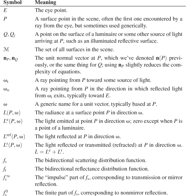
To discuss light transport, we need to use quite a lot of notation, which we’ll reuse in subsequent chapters. We summarize these symbols in Table 29.1, even though some are given full definitions only later in the chapter.
For mathematical convenience, we’re going to consider a scene that is finite, in the sense that it’s contained within some sufficiently large sphere around the origin; the interior of this sphere we’ll assume to be coated with a nonreflective material so that all light hitting it is absorbed. In a real scene, once light “leaves” the scene, we ignore it. But for this chapter, it’s very useful to have a ray-casting function that takes a point P and direction d and returns the first surface point Q along the ray starting at P and going in direction d. If the scene isn’t surrounded by the large sphere, then a ray headed “out of the scene” doesn’t hit anything, and the ray-casting function’s value is not defined. So the large black sphere is completely for mathematical convenience, and it has no impact on the actual transport of light.
To keep the notation simple, we’re going to further assume that we’re studying a steady-state situation, one in which there is no time dependence: The luminaires have all been illuminated for long enough to allow light to scatter throughout the scene and reach a steady state. Furthermore, we’re going to ignore the wavelength dependence, and study just radiance rather than spectral radiance.
Thus, our starting point is a collection of surfaces whose union is the set M of all surface points in the scene (including the large enclosing black sphere). For each point P ![]() M, we also know fr(P, ωi, ωo), the bidirectional reflectance distribution function at P, which describes how much light arriving at P traveling in direction –ωi becomes light leaving in direction ωo (see Chapter 26 for the formal definition). The symbols ωi and ωo will be reserved, for this section, to be unit vectors that point in the same half-plane as the normal vector nP at P, that is, ωi · nP ≥ 0 and ωo · nP ≥ 0.
M, we also know fr(P, ωi, ωo), the bidirectional reflectance distribution function at P, which describes how much light arriving at P traveling in direction –ωi becomes light leaving in direction ωo (see Chapter 26 for the formal definition). The symbols ωi and ωo will be reserved, for this section, to be unit vectors that point in the same half-plane as the normal vector nP at P, that is, ωi · nP ≥ 0 and ωo · nP ≥ 0.
In addition to the scene geometry and reflectance, we assume that we’re given the illumination in the scene, described by the emitted radiance at every point of every luminaire, in every direction; in other words, we’re given a function
where Le(P, ω) denotes the emitted radiance leaving the point P in direction ω, the radiance you’d measure if every other luminaire and surface in the scene were removed, so that no light at all arrived at the point P, and hence none was reflected.
As we said above, we’ll also assume we have a ray-casting function (see Figure 29.1),
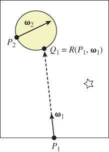
where R(P, ω) is the first point hit by a ray starting at P in direction ω. If ω · nP ≤ 0, then R(P, ω) = P, that is, a ray into a shape hits the shape immediately. If ω · nP > 0, then R(P, ω) is the point we see by looking in direction ω from P. More precisely, R(P, ω) is the farthest point Q on the ray from P in direction ω with the property that all points of the ray strictly between P and Q are in empty space.
The algorithmic representation of the ray-casting function and the associated visibility function—see Exercise 29.1—is the subject of Chapters 36 and 37, but you’ve already seen basic examples in Chapter 15.
With our assumptions clearly characterized, we can now analyze the light transport in our scene.
29.2.1. The Rendering Equation, First Version
Consider once again the reflectance equation, Equation 26.80, rewritten without time or wavelength dependence:
This expresses the radiance reflected at point P in outward direction ωo in terms of the light arriving at P in other directions.
If P happens to be a point of a luminaire, light may also leave P in direction ωo because it is emitted at P rather than because it is reflected from there; that is,
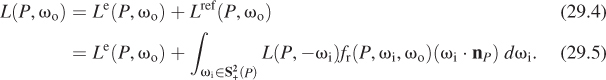
This is a basic version (e.g., it handles only reflection) of the rendering equation, which characterizes the function L, given the functions Le and fr. It was first described in computer graphics by Kajiya [Kaj86] and Immel et al. [ICG86], in slightly differing forms. It is completely analogous to similar equations developed in subjects like radiative transfer. While we’ll concentrate on Kajiya’s description and derivation in subsequent chapters, the form presented by Immel et al. is particularly well suited to the “sampling” needed in Monte Carlo rendering.
You’ll notice that the unknown radiance function L appears on both sides of the equation, once under an integral, just as the unknown function h appears on both sides of the differential equation
once within a derivative. Equation 29.4 is called an integral equation, and solving such an equation is generally more difficult than solving a differential equation. The next chapter discusses various approaches to finding approximate solutions.
Equation 29.4 expresses the radiance function L, considering both the radiance leaving the point P and the radiance arriving there. Arvo [Arv95] calls the first of these the surface radiance and the second the field radiance. The rendering equation tells us how to compute surface radiance from field radiance, because it’s restricted to the case where ωo · nP > 0. But to evaluate the right-hand side, we must know how to compute the field radiance as well.
The idea that “closes the loop” in this equation is that any light arriving at a point P, traveling in direction –ωi, must have departed from some other point Q ![]() M traveling in direction –ωi. The point Q must be the point visible from P in direction ωi. These observations allow us to write the transport equation:
M traveling in direction –ωi. The point Q must be the point visible from P in direction ωi. These observations allow us to write the transport equation:
for any ωi with ωi · nP > 0.
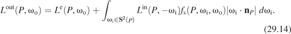
Substituting Equation 29.7 into Equation 29.4, we get the form of the rendering equation that’s most useful in practice:
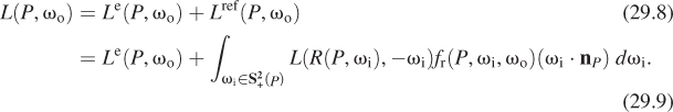
This equation expresses the surface radiance function defined on all surfaces in the scene, in terms of the known luminaires (Le), and an integral of the known BRDFs of all surface points (fr), the ray-casting function R, and the surface radiance itself.
29.3. A Peek Ahead
The rendering equation is very nice and self-contained, but how do you do anything with it? Let’s take a quick look ahead at code from Chapter 32 to see. The large-scale structure of a basic path tracer is:
1 foreach pixel (i, j)
2 C = location of pixel on image plane
3 r = ray from eye to C
4 image[i, j] = pathTrace(r, true)
Listing 29.1 shows the central pathTrace procedure for such a path tracer. Given a ray (i.e., a point U and a direction ω) this procedure traces a ray into the scene and hits at some point P, and then estimates either L(P, –ω) or Lref(P, –ω), depending on the boolean isEyeRay. The point P is represented by the variable surfel (for “surface element”) in the program.
Listing 29.1: The core procedure in a path tracer.
1 Radiance3 App::pathTrace(const Ray& ray, bool isEyeRay) {
2 Radiance3 radiance = Radiance3::zero();
3 SurfaceElement surfel;
4
5 float dist = inf();
6 if (m_world->intersect(ray, dist, surfel)) {
7 if (isEyeRay)
8 radiance += surfel.material.emit;
9
10 radiance+= estimateDirectLightFromPointLights(surfel, ray);
11 radiance+= estimateDirectLightFromAreaLights(surfel, ray);
12 radiance+= estimateIndirectLight(surfel, ray, isEyeRay);
13 }
14 return radiance;
15 }
As you can see, the outgoing radiance at P is the sum of the emitted light (surfel.material.emit) and the light reflected at P, estimated in the last three procedures. The first estimates the light arriving directly from point sources that’s reflected at P; the second the light directly from area luminaires that’s reflected at P; and the third all other light. Thus, the term L(P, –ωi) in the rendering equation has been split into a sum of three terms.
The first of these terms is computed (see Listing 29.2) by converting the integral over all possible incoming directions into a sum over the point luminaire sources. This change of domain in the integral means we have to alter the integrand as well, using the change of variable from Section 26.6.5.
Listing 29.2: Reflecting illumination from point lights.
1 Radiance3 App::estimateDirectLightFromPointLights(surfel, ray){
2 Radiance3 radiance(0.0f);
3 for (int L = 0; L < m_world->lightArray.size(); ++L) {
4 const GLight& light = m_world->lightArray[L];
5 // Shadow rays
6 boolean visible = m_world->lineOfSight(surfel.geometric.location +
7 surfel.geometric.normal * 0.0001f,
8 light.position.xyz())
9 if (visible){
10 Vector3 w_i = light.position.xyz() - surfel.shading.location;
11 const float distance2 = w_i.squaredLength();
12 w_i /= sqrt(distance2);
13 // Attenuated radiance
14 const Irradiance3& E_i = light.color / (4.0f * pif() * distance2);
15
16 radiance += (surfel.evaluateBRDF(w_i, -ray.direction()) *
17 E_i * max(0.0f, w_i.dot(surfel.shading.normal)));
18 }
19 }
20 return radiance;
21 }
As you can see, the procedure loops through all the point luminaire sources, and for each one, it checks whether the source is visible from P, using m_world->lineOfSight(), the implementation of the visibility function for the world we’re rendering. The reflected radiance is computed as a product of the BRDF, the dot product ωi · nP, and a term Ei, which is the incoming radiance adjusted by the change-of-variable factor mentioned above.
The second term is similar, involving estimates of how area luminaires are reflected. The third term is the most interesting, however. Before we look at it, we need one more bit of mathematics (which we’ll develop extensively in Chapter 30).
The idea is this: The integral of any function h over any domain D is the product of the average value of h on that domain with the size of the domain. When the domain is the interval [a, b], the size is b – a; when the domain is a unit hemisphere, the size is 2π, etc. The “average value” can be estimated by evaluating h at n points of the domain and averaging. As n gets large, the estimate gets better and better. But even n = 1 works! That is to say, we can estimate the integral of h over the domain D by evaluating h(x) for a randomly chosen point x ![]() D and multiplying by the size of D. The estimate won’t generally be very good, but if we repeat the estimation procedure multiple times, the average will be quite a good estimate.
D and multiplying by the size of D. The estimate won’t generally be very good, but if we repeat the estimation procedure multiple times, the average will be quite a good estimate.
We’ll apply this to the situation where h is the integrand in the reflectance equation, and D is the upper hemisphere. Let’s look at the code (see Listing 29.3).
Listing 29.3: Estimating the indirect light scattered back along a ray.
1 Radiance3 App::estimateIndirectLight(surfel, ray, bool isEyeRay){
2 Radiance3 radiance(0.0f);
3 // Use recursion to estimate light running back along ray from surfel that arrives from
4 // INDIRECT sources, by making a single-sample estimate of the arriving light.
5
6 Vector3 w_o = -ray.direction();
7 Vector3 w_i;
8 Color3 coeff;
9
10 if (surfel.scatter(w_o, w_i, coeff)) {
11
12 newRay = Ray(surfel.geometric.location, w_i).bumpedRay(
13 0.0001f * sign(surfel.geometric.normal.dot(w_i));
14 // the final "false" makes sure that we do not include direct light.
15 radiance = coeff * pathTrace(newRay, surfel.geometric.normal), false);
16 }
17 return radiance;
18 }
Without worrying too much about the details, what’s happening here is that we’re picking a random direction w_i, using scatter, on the outgoing hemisphere. We’re then using PathTrace to estimate the radiance arriving at P from that direction, that is, we’re estimating L(P, –ωi). The coefficient by which we multiply this radiance includes the area of the hemisphere and an adjustment for the fact that we did not pick our direction uniformly from all possible directions, but instead biased our choice based on the BRDF, for reasons you’ll learn about in Chapter 30.
To summarize: The recursive nature of the rendering equation is exactly reflected in the recursive nature of the program. You might reasonably ask whether the recursion will ever terminate, since there seems to be no stopping condition. The answer is yes, because of the design of the scatter procedure: If a surface’s hemispherical reflectance is 0. 7, then 30% of the time scatter will return false and the recursion will terminate. The other 70% of the time the coefficient coeff is adjusted to take into account the probability of nonscattering.
29.4. The Rendering Equation for General Scattering
In formulating the rendering equation, we assumed that our scene contained only reflective materials rather than ones that could transmit light, or participating media like fog that can scatter light as it passes through them.
We’ll now generalize to handle transmissive materials as well. This will require almost no new concepts, but we’ll need to slightly revise the way we represent the radiance in a scene. A further revision is needed to handle participating media, which we will not discuss here. Instead, we’ll consider just one special case, in which light is attenuated by absorption as it passes through a medium but is never scattered in any new direction. More general models of scattering, discussed briefly in Chapter 27, can be used to generate quite striking renderings like that shown in Figure 29.2 from 1987, one of the earliest high-quality synthetic images of participating media.
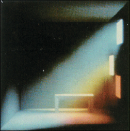
Figure 29.2: Rendering with a participating medium (dusty air). (Courtesy of Holly Rushmeier, ©1987 ACM, Inc. Reprinted by permission.)
The critical problem, when we want to include transparency into the rendering equation, is that a pair (P, ω) ![]() M × S2 is no longer associated to a unique radiance value.
M × S2 is no longer associated to a unique radiance value.
Because we are only doing surface rendering rather than volume rendering (i.e., we’re ignoring participating media), we only care about L(P, ω) for points P that are on some surface. That surface must have a surface normal n at P. We can therefore define L(P, ω, n) by the rule that if ω and n have a positive dot product, then L(P, ω, n) represents the radiance leaving the surface in direction ω; if their dot product is negative, then it represents the radiance arriving at the surface in direction ω. By using either the unit outward surface normal or its opposite as n, we can handle both reflection and transmission. In practice, this turns into an additional if statement at every ray-surface interaction: A surface element has two sides (one with a normal pointing each way), and we treat the vector ω differently depending on whether it points in the same or the opposite ![]() half-space as the normal vector to the “side.” In mathematical terms, we can say that L is defined on the orientation double cover [Lee09] of the set of all scene surfaces.
half-space as the normal vector to the “side.” In mathematical terms, we can say that L is defined on the orientation double cover [Lee09] of the set of all scene surfaces.
The three-argument version of L is awkward to write. As an alternative, we can replace L altogether with two new functions: (P, ω) ![]() Lin(P, ω) and (P, ω)
Lin(P, ω) and (P, ω) ![]() Lout(P, ω), which represent light arriving at P traveling in direction ω and light leaving P in direction ω, respectively; these are Arvo’s field and surface radiance functions. The reflectance equation then becomes a scattering equation:
Lout(P, ω), which represent light arriving at P traveling in direction ω and light leaving P in direction ω, respectively; these are Arvo’s field and surface radiance functions. The reflectance equation then becomes a scattering equation:
where five things have changed.
• The integral is now over all directions of incoming light.
• The result is now Lr rather than Lref (recall that Lr denotes light either reflected or transmitted).
• The BRDF fr has been replaced with the BSDF fs.
• The dot product now has an absolute value.
• The annotations “in” and “out” have been added to the radiance and scattered radiance.
The transport equation now links incoming and outgoing light. We write the equation in two forms, one suitable for use in ray tracing, the other for use in photon mapping. The distinction is simply one of tracing rays in the direction of photon propagation or in the opposite direction. The version used in raytracing is this:
while the one that’s useful in photon mapping is this:
Dividing the radiance field into two parts has further advantages. When we write the radiance field this way, it naturally extends to all points P rather than limiting us to those points that lie on surfaces—we define radiance at (P, ω) for a nonsurface point P by letting Q = R(P, – ω), and setting
which results in radiance that’s constant along rays in empty space. In Equation 29.13, we defined L(P, ω) rather than Lin or Lout because at points of empty space, these two functions agree; they only differ at points of M.
The rendering equation now becomes
The changes we’ve made to incorporate transmission seem fussy and likely to lead to code with multiple cases. In practice, however, they have almost no effect. That’s partly because of the restricted model of scattering we use in representing materials in Chapter 32: Scattering at a surface point consists of a small number of impulses and an otherwise diffuse or glossy reflectance-scattering pattern. (Recall that an impulse is a phenomenon that is similar to mirror reflection or Snell-Fresnel refraction, where radiance arriving along one ray scatters out along just one or two other rays.) In particular, in the general rendering equation, the part of the integral representing transmission degenerates to something far simpler: We look at the radiance arriving along one particular ray, multiply it by a constant representing how much light is transmitted, and add the result to the outgoing radiance.
29.4.1. The Measurement Equation
Typically a renderer takes a scene description as input, and produces an image—a rectangular array of values—as output. These values might just be RGB triples in some fixed range, or they might be RGB radiance values representing radiance in W m–2 sr–1, or something else. In general, a particular pixel value represents the result of a measurement process. For a typical digital camera, the red measurement, for one pixel, represents the total charge accumulated in one cell of a CCD device. For a synthetic camera, it might represent the integral of irradiance in the red portion of the spectrum over the rectangular corresponding to one pixel on the image plane. Or it might represent a weighted integral of this irradiance over a disk slightly larger than the rectangle usually associated to a pixel so that radiance along a single ray contributes to the value of more than one pixel in the final image. We express this idea by associating to each pixel ij a sensor response Mij, which converts radiance along any ray into a numerical value that can be summed over all rays to get the sensor value. That is to say, we posit that the measurement mij associated to pixel ij is computed as
where U is the image plane. This is a purely formal description of the measurement process. The critical thing is that Mij is zero except for points in a small area and directions in a small solid angle. For a camera with a small pinhole aperture, for instance, Mij(P, ω) is nonzero only if both of the following are true.
• The ray t ![]() P + tω passes through the pinhole.
P + tω passes through the pinhole.
• P is within the part of the image plane associated to pixel ij.
In this case, the radiance Lin(P, –ω) arriving at P is multiplied by the sensor response associated to this ray.
For a real physical sensor, the sensor response is called flux responsivity and has units of W–1. Since the radiance is in W m–2 sr–1, and we integrate out square meters and steradians, this makes the measurement mij unitless.
For a typical sensor, Mij has a form that’s independent of the pixel ij. For example, it might have the constant value 1 on a small rectangle representing the pixel, and zero elsewhere. While the region on which it takes the value 1 changes with ij, the form of the function doesn’t change.
When we consider the space of all paths along which light might travel in a scene, from the point of view of rendering, some are more important than others. In particular, the paths that end up entering the virtual camera matter more to us than do those that end up absorbed in some distant and invisible part of the scene. Thus, the function Mij can help us decide which paths might be worth examining. Because of this, it’s been called the importance function [Vea96].
29.5. Scattering, Revisited
In the introduction, we talked (broadly) about two types of scattering. The first is mirrorlike: Radiance arriving from some direction ωi leaves in a single direction ωo, perhaps after attenuation by some factor 0 ≤ c ≤ 1. The two main examples of mirrorlike reflectance are (a) mirrors, and (b) Snell’s-law refraction. The second type of scattering is diffuselike scattering, in which radiance arriving in some direction is scattered over a whole solid angle of directions (perhaps uniformly with respect to angle—the Lambertian case—or perhaps nonuniformly). In this second kind of scattering, the outgoing radiance in a direction ωo due to radiance along a single ray in direction –ωi is infinitesimal: To get a nonzero outgoing radiance, we must sum radiance scattered from a whole solid angle of incoming directions; the integral in the rendering equation expresses exactly this. For the integral formulation to apply to the first part requires the fiction of “infinite values” for fs akin to delta functions.
We can treat the process of converting incoming radiance to outgoing radiance as an operation K that takes the incoming radiance and scattering functions as input and produces the outgoing radiance Lout = K(Lin, fs). What we’ve said in the previous paragraph is that fs should be written as a sum ![]() , the first being the “finite part” and the second being the “impulse part”; the rule for combining the field radiance with the finite part to get the surface radiance can then be legitimately expressed as an integral:
, the first being the “finite part” and the second being the “impulse part”; the rule for combining the field radiance with the finite part to get the surface radiance can then be legitimately expressed as an integral:
In the opaque (i.e., reflection-only) case, the integral would be over a hemisphere, and we’d write fr instead of fs.
The rule for combining the incoming radiance with the impulse part has the form
where H(ωo) is the (finite) set of directions ωi that undergo mirrorlike scattering at P to direction ωo, and ![]() denotes the constant by which incoming radiance is scaled to produce outgoing radiance, which we’ve previously called the magnitude of the impulse.
denotes the constant by which incoming radiance is scaled to produce outgoing radiance, which we’ve previously called the magnitude of the impulse.
![]() There’s a slight subtlety here. The form given in Equation 29.17 is only valid if Lin is continuous at (P, –ωi). Otherwise, the value must be determined by a limit. As far as we know, this detail is generally ignored in graphics, perhaps because almost all physical processes involve convolution, and convolution tends to produce continuous functions. That is to say, perhaps our pure mathematically modeled Lin has a discontinuity, but if we were in the real world, things like volumetric scattering would tend to make it actually continuous. Any picture whose appearance depended on the discontinuity of Lin would be nonphysical anyhow!
There’s a slight subtlety here. The form given in Equation 29.17 is only valid if Lin is continuous at (P, –ωi). Otherwise, the value must be determined by a limit. As far as we know, this detail is generally ignored in graphics, perhaps because almost all physical processes involve convolution, and convolution tends to produce continuous functions. That is to say, perhaps our pure mathematically modeled Lin has a discontinuity, but if we were in the real world, things like volumetric scattering would tend to make it actually continuous. Any picture whose appearance depended on the discontinuity of Lin would be nonphysical anyhow!
29.6. A Worked Example
Consider the situation in Figure 29.3. The surface is 50% Lambertian and 30% a mirror reflector (so 20% of arriving light is absorbed). We’ll compute the light reflected from the point P = (0, 0, 0) under two different lighting conditions.
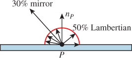
Figure 29.3: Scattering example: a 50% matte reflector that’s also 30% mirror-reflective, but not transmissive.
1. The surface is bathed in light from all points of the postive-x hemisphere (see Figure 29.4). The radiance Lin(P, –ωi) is 6 W m–2 sr–1 for all ωi with ωi · [1 0 0]T ≥ 0.
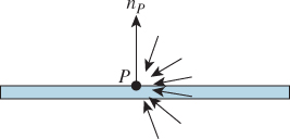
2. The surface is illuminated by a uniformly radiating sphere (see Figure 29.5) of radius r < 1 at position Q = (1, 1, 0); the total power of the luminaire is 10 W.

Figure 29.5: The point P is illuminated by a tiny, uniformly emitting, spherical lamp at location Q.
We’ll examine the behavior of the second case as r ![]() 0 as well.
0 as well.
In each case, we’ll compute the reflected radiance in the direction ωo = S([–1 1 0]T).
We start with situation 1. Let’s begin by computing the diffusely reflected light. This is
Rewriting ωi in polar coordinates, (x, y, z) = (cos θ sin φ, cos φ, sin φ sin φ), the radiance field L(P, –ωi) is zero unless x > 0, that is, cos θ > 0, so we can restrict to – ![]() ≤ θ ≤
≤ θ ≤ ![]() . Similarly, since we’re only considering reflectance, we can restrict to 0 ≤ φ ≤
. Similarly, since we’re only considering reflectance, we can restrict to 0 ≤ φ ≤ ![]() . Thus, our integral becomes
. Thus, our integral becomes
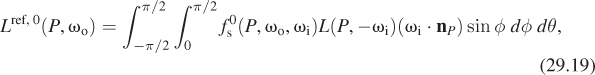
where the factor of sin φ comes from the change to polar coordinates. Within this restricted domain, the value of L is the constant 6, so the integral becomes

where we’ve replaced the dot product with cos φ. Finally, the finite part of the BSDF is the constant ![]() sr–1, so the reflected radiance becomes
sr–1, so the reflected radiance becomes
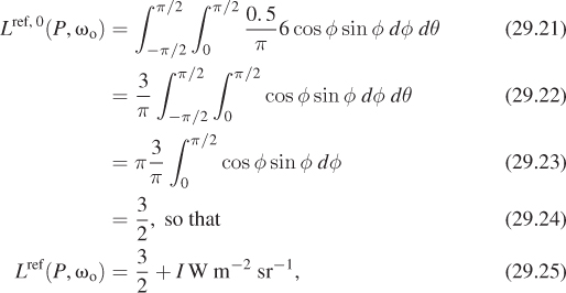
where I is the impulsively reflected (i.e., mirror-reflected) radiance. Since the surface is 30% mirror-reflective, the incoming radiance of 6 W m–2 sr–1 is multiplied by the magnitude 0. 3 to get the outgoing mirror-reflected radiance, 1.8 W m–2 sr–1. Thus, the total reflected radiance is ![]() + 1. 8 W m–2 sr–1 = 3. 3 W m–2 sr–1.
+ 1. 8 W m–2 sr–1 = 3. 3 W m–2 sr–1.
As a result, we’ve converted the handling of an impulse in the scattering function from an integral to a simple multiplication by a constant, the impulse magnitude.
Now, as we look at the second situation, with illumination provided by a 10 W radiating small sphere, we’ll see how each term (the diffuse and the impulse) behaves when there’s an “impulse” in the incoming light field (i.e., a point light), by seeing what happens as the radius of the sphere approaches zero.
As we showed in Section 26.7.3, a uniformly radiating sphere of radius r and total power Φ produces radiance ![]() along every outgoing ray, and subtends a solid angle approximately
along every outgoing ray, and subtends a solid angle approximately ![]() at a point at distance R, with the approximation growing better and better as R increases or r decreases.
at a point at distance R, with the approximation growing better and better as R increases or r decreases.
The integral to compute the Lambertian-reflected light from this small spherical source is essentially the same as the one above, except that instead of integrating over all directions ωi = [x y z]T with x ≥ 0, we now must integrate over just the small solid angle Ω subtended at P by the small spherical source. So
where I as before represents the impulse-reflected radiance and ![]() again is the constant function 0. 5/π sr–1 Furthermore, for ωi in the solid angle subtended by the luminaire, ωi · n(P) is well approximated by u · n(P), where u is the unit vector from P to the center Q of the radiating sphere, that is,
again is the constant function 0. 5/π sr–1 Furthermore, for ωi in the solid angle subtended by the luminaire, ωi · n(P) is well approximated by u · n(P), where u is the unit vector from P to the center Q of the radiating sphere, that is, ![]() . Since the normal n(P) points in the y-direction, this dot product is just
. Since the normal n(P) points in the y-direction, this dot product is just ![]() . Hence,
. Hence,
The radiance along each ray is the constant ![]() , so this becomes
, so this becomes
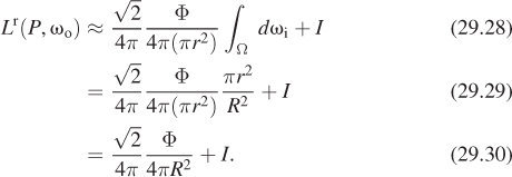
Since ![]() and Φ = 10, we get that the reflected radiance is
and Φ = 10, we get that the reflected radiance is ![]() . Notice that this approximation of Equation 29.28 is independent of r so that even as the spherical luminaire shrinks to a point, the reflected radiance remains the same.
. Notice that this approximation of Equation 29.28 is independent of r so that even as the spherical luminaire shrinks to a point, the reflected radiance remains the same.
![]() The constancy of the reflected radiance depends on two things: the assumption that the dot product ωi · n(P) can be approximated by u · n(P), and the fact that the finite portion of the scattering function is constant. The first of these is justified because we’re letting r approach zero. The second is not true for a general BSDF. But if
The constancy of the reflected radiance depends on two things: the assumption that the dot product ωi · n(P) can be approximated by u · n(P), and the fact that the finite portion of the scattering function is constant. The first of these is justified because we’re letting r approach zero. The second is not true for a general BSDF. But if ![]() is continuous, as it is in all the BSDFs that we consider, then the mean value theorem for integrals tells us that the integral we wish to compute is equal to
is continuous, as it is in all the BSDFs that we consider, then the mean value theorem for integrals tells us that the integral we wish to compute is equal to
for some ω*i in Ω. As the area of Ω goes to zero, this vector ωi* must approach u, so the integral approaches
To summarize the preceding argument, a point luminaire of power Φ, in direction ωi from P, at distance R, produces reflected radiance (from the nonimpulse portion of scattering) in direction ωo in the amount
Finally, let’s consider the impulse reflection of the very small spherical source. The radiance leaving each point of the luminaire is again![]() . Because ωi points to a point of the luminaire, the radiance arriving in direction –ωi is
. Because ωi points to a point of the luminaire, the radiance arriving in direction –ωi is ![]() ; to get the outgoing radiance in the mirror-reflected direction ωo, we multiply by the impulse value 0.3 so that the outgoing radiance due to mirror reflection of the very small spherical source is 0.3
; to get the outgoing radiance in the mirror-reflected direction ωo, we multiply by the impulse value 0.3 so that the outgoing radiance due to mirror reflection of the very small spherical source is 0.3 ![]() . Notice that this depends on the value of r! As the size of the luminaire decreases, the radiance emitted must increase to keep the total power the same, with the result that the mirror-reflected radiance also increases without bound. If we try to take a limit, we end up with an answer that includes ∞, which is unsatisfactory.
. Notice that this depends on the value of r! As the size of the luminaire decreases, the radiance emitted must increase to keep the total power the same, with the result that the mirror-reflected radiance also increases without bound. If we try to take a limit, we end up with an answer that includes ∞, which is unsatisfactory.
There are several possible ways to address this problem.
1. Assert that no eye ray that we trace will ever “just happen” to hit a point luminaire, so this is a probability-zero event, and we can ignore the infinity that would arise if this event happened.
2. Say that for the sake of reflecting from diffuse surfaces, point lights are points, but for the sake of specular reflections, they have a nonzero radius r, which must be chosen by the user. Note that this makes the world in which we’re trying to simulate light transport internally contradictory.
3. Say that point lights are in fact small spheres of a known radius, r, but that we’ll restrict our scene to be sure that the distance from a point luminaire to any surface is much greater than r so that the diffusely reflected light can be very well approximated by treating the sources as point sources, but mirror-reflected light must be computed using r.
4. Observe that when we include both point lights and mirror reflections, both of which are approximations of physical phenomena made for convenience, the mathematics becomes intractable, and hence we’ll abandon one or both.
Each of these approaches has its merits, although we prefer approach 3 to approach 2 (even though they both may result in identical programs). In Chapter 32, we choose the first option: We simply ignore mirror-reflected point lights.
29.7. Solving the Rendering Equation
It’s natural to ask, having derived the rendering equation, how to solve it. That is to say, if we know the scene geometry and materials and illumination, how can we compute L(P, ω) for any point P and any vector ω, or for every P and every ω? We’ve already given you a taste of the answer in discussing a path tracer. But the general topic is the subject of the next three chapters. Because integration is central to the rendering equation, the first discusses probability and Monte Carlo integration. The second describes the ideas behind several techniques for solving the rendering equation. The third gives an implementation of two renderers. One of the shocking things is how very short the two programs are, given the length of this chapter and the next three. That brevity is partly due to the use of libraries for things like visibility testing, basic linear algebra, and material representation. But as you’ll see, it’s also due to the simplicity of basic Monte Carlo integration.
29.8. The Classification of Light-Transport Paths
In the course of the Monte Carlo integration used to estimate solutions to the rendering equation, we’ll break up the integrals of the rendering equation into different parts—sometimes by breaking up the domain of integration into the categories of “directions in which we see luminaires” and “other directions,” and sometimes by breaking up the integrand into a sum of a finite part and an impulse part, usually as a means of distinguishing between things like point luminaire and area luminaires, or between mirror reflections and diffuse reflections.
Because of this distinction in treatment, it’s useful to be able to discuss the path that light took in getting from the luminaire to the receiver (a light path), or its reverse, the path we traced from the eye to eventually reach the light source (an eye path). Heckbert [Hec90] used a notation that’s now universally accepted:1 L denotes a luminaire, E the “eye,” S a specular reflection, and D a diffuse reflection. Thus, LDE represents light that left the source, scattered from a diffuse surface, and reached the eye. Conventional regular-expression notation is useful here, with + used to indicate “one or more,” * for “zero or more,”? for “zero or one,” parentheses for grouping, and | for “or,” so that L(D|S)E denotes a one-bounce path from a source to the eye that involves either a diffuse or specular reflection, while LD+E is a path involving one or more diffuse bounces.
1. Hanrahan [JAF+01] attributes this notation to Shirley, who claims [Shi10] that he’s uncertain who first used it.
(a) Write the notation for light that undergoes one or more diffuse bounces, and then a final specular bounce before reaching the eye.
(b) A very basic ray tracer might consider rays from the eye that undergo only repeated specular bounces, followed by zero or one diffuse bounce, before reaching the light. Write the notation for the path traveled by the light, from luminaire to eye.
Note that the notation describes a sequence of scattering events, not just the path. In the case of the half-mirror surface we just discussed, light could travel from a luminaire to the surface, be mirror-reflected, and reach the eye; it could also travel from the source, be diffusely scattered, and reach the eye. The light energy in the two cases travels along the same path, but the first is described by LSE while the second is described by LDE.
There are extensions that are fairly common. Veach uses D to mean Lambertian, G for any kind of glossy reflection, S for perfectly specular, and T for transmission, for instance [Vea97].
We can use this notation to characterize certain rendering algorithms in terms of the eye paths that they consider, following Hanrahan [JAF+01]:
• Appel’s ray-casting algorithm: E(D|G)L
• Recursive ray tracing (Whitted): E[S*](D|G)L
• Path tracing (Kajiya): E[(D|G|S)+)D|G)]L
• Radiosity: ED*L
Recursive ray tracing considers only light that’s diffusely or glossily reflected, and then mirror-reflected to the eye. Radiosity only handles diffuse reflections. And Appel’s ray-casting algorithm considers only direct lighting.
29.8.1. Perceptually Significant Phenomena and Light Transport
We conclude this largely mathematical chapter with a discussion of things we notice when we look at the world, for these phenomena—the things we take the trouble to name—are the things we must render effectively if we want to make compelling images. They thus serve as a guide to developing rendering algorithms.
The first phenomenon is the shadow. Figure 29.6 shows a hard shadow, created by a luminaire (the sun) that subtends a very small solid angle. The light from the sun is obstructed by the sharp edge of an object. Figure 29.7 shows a soft shadow. Soft shadows can be caused by many things: If the shadowing object is not sharply defined (e.g., a furry animal), the shadow may have no distinct edge, even if it’s cast by a point luminaire. If the shadow is cast by a very small object, diffraction effects may dominate and effectively soften the shadow. But most often, soft shadowing is caused by nonpoint luminaires: A point on the receiving surface may be invisible from every point on the light source, in which case it’s in the umbra, or it may be visible from just some of the points of the luminaire, in which case it’s in the penumbra, or it may be visible to all points of the source, in which case it’s not shadowed at all. To be more precise: A point P is in the penumbra if the set of points of the luminaire, L, visible from P when the occluder is removed, is different from the visible set when the occluder is present. Thus, if L is a typical incandescent lightbulb, we don’t require that every point of the bulb be visible from P (which never happens), but only that every point that could be visible from P actually is visible.
The next important phenomenon is boundaries such as the contours discussed in Chapter 5. Boundaries between objects, between materials in a single object, etc., are all significant. (Indeed, shadow edges are yet another example of boundaries.)
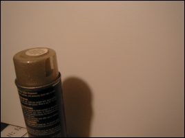
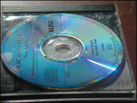
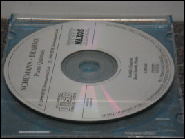
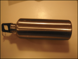
Many surface properties are revealed through reflection of light. Under point illumination, diffractive objects like the surface of the CD in Figure 29.8 clearly reveal their reflectance structure; under area luminaires, the reflection is less focused but still shows the characteristic rainbow pattern (see Figure 29.9). Less extreme than diffraction are the stretched-out highlights that appear on brushed-metal surfaces (see Figure 29.10); the alignment of the brush marks generates these in much the same way that ripples on a pond generate an extruded reflection of moonlight.
And of course, for more common scattering functions, phenomena like edge highlights, generated by very glossy materials with high curvature (see Figure 29.11), are commonplace.

Figure 29.11: The bright line along the edge of the bookshelf results from the glossy reflection of sunlight.
Polarization phenomena are less obvious in general, although anyone who has worn polarized sunglasses knows that mirror-reflected light tends to be somewhat polarized, and therefore can be attenuated by the polarizing lens in the sunglasses.
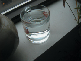
Caustics (see Figure 29.12) are bright areas that arise from the focusing of illumination by curved surfaces, through either reflection or refraction. Typically they are produced by point sources or small area sources like the sun. Figure 29.13 shows how caustics weaken or disappear under more diffuse illumination.
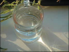
![]() Assuming for the moment that most caustics arise from sunlight, that is, from light arriving on essentially parallel rays, caustics will, in general, appear close to the curved surfaces that cause them. Figure 29.12 suggests the reason: You can see several rays meeting at a bright spot, but beyond that spot, the rays diverge. Since caustics depend on convergence, once you are sufficiently distant from a surface (roughly, the maximum radius of curvature of the surface) the caustics can no longer appear. By studying the focal points of a surface (places at which nearby normal rays meet), you can determine how likely a surface is to cast a caustic on some distant object under random parallel illumination.
Assuming for the moment that most caustics arise from sunlight, that is, from light arriving on essentially parallel rays, caustics will, in general, appear close to the curved surfaces that cause them. Figure 29.12 suggests the reason: You can see several rays meeting at a bright spot, but beyond that spot, the rays diverge. Since caustics depend on convergence, once you are sufficiently distant from a surface (roughly, the maximum radius of curvature of the surface) the caustics can no longer appear. By studying the focal points of a surface (places at which nearby normal rays meet), you can determine how likely a surface is to cast a caustic on some distant object under random parallel illumination.
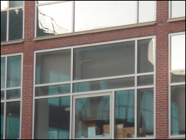
There’s a dual phenomenon to caustics: Eye rays meeting a curved surface may converge on a single point, or a small range of points. A magnifying glass is designed to take advantage of this phenomenon, for instance, but it also appears in less intentional settings. For instance, the reflections of the blue windows in Figure 29.14 appear somewhat wavy and distorted because of the curvature of the windows in which they’re reflected.
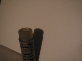
Transmission of light through transparent media also generates refractive phenomena, like the offset in the top and bottom parts of the red pen in Figure 29.15. Because spatial continuity (things that are straight should appear straight, things in a regular pattern should appear regular, etc.) is easily noticed, its interruption by refraction is perceptually significant.

If you are reading this indoors, then most of the light that you are seeing has been reflected multiple times. You can verify this by standing in an empty room with painted walls, illuminated by a single bulb. If you place a black occluder next to the bulb, some portion of the room will be “in shadow,” but nonetheless remains remarkably bright. The importance of this multiply reflected light is not well measured by computing energies, because of the logarithmic sensitivity of the eye: Even comparatively dark areas are easy for us to see; these darker areas are ones where indirect illumination has taken multiple attenuating bounces. Even though little energy from them is reaching the eye, we can easily detect variations on surfaces, such as the pattern on a carpet in a dark corner of a room.
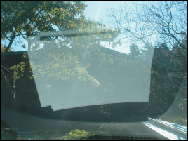
These variations in dark regions can, however, be lost in the presence of other light. Figure 29.16 shows how the view through a car window can be masked by reflected light from papers on the dashboard.
Keep these examples in mind as you read about rendering algorithms, and ask yourself which of them each algorithm is capable of replicating.
29.9. Discussion
The key ideas in this chapter are the reflection equation and the transport equation, which combine to form the rendering equation, and the measurement equation, which is added as a final step in the process of image formation. Equally important is the notion of dividing various phenomena into “impulse” and “finite” pieces. This division applies to the BSDF, where impulses include mirror reflection and Snell’s-law refraction, and to luminaires, where point lights act as a kind of impulse in the illumination. Such impulses require that we regard integrals with a skeptical eye, because integrals of finite pieces can be reliably estimated with Monte Carlo methods, as we’ll see in the next few chapters, while those involving impulses must be treated separately.
The physical formulation of light transport is central to rendering, but it’s also worth understanding the phenomena, that is, the human-perceived aspects, of light transport. The tiny “rainbows” cast by a chandelier on the walls of a well-lit room are insignificant in the total illumination by physical measures, but to a person sitting in the room, they are important characteristics that attract attention. Understanding these phenomena helps us understand which aspects of physical light transport may have greater impacts on the perceived correctness of an image.
29.10. Exercise
Exercise 29.1: Show that if you have the ray-casting function R, then you can build a visibility function V : ![]() ×
× ![]()
![]() 0, 1, where V(P, Q) is 1 if all points of the line segment from P to Q that are strictly between the ends are in empty space, and is 0 otherwise. Informally, V(P· Q) is 1 when Q is visible from P (and vice versa). Note that according to our definition, V(P, P) is always 1. You may assume that you have a mechanism for perfect equality testing of points.
0, 1, where V(P, Q) is 1 if all points of the line segment from P to Q that are strictly between the ends are in empty space, and is 0 otherwise. Informally, V(P· Q) is 1 when Q is visible from P (and vice versa). Note that according to our definition, V(P, P) is always 1. You may assume that you have a mechanism for perfect equality testing of points.