
Chapter 27. Materials and Scattering
27.1. Introduction
This chapter is about the way we model the interaction of light with objects. The first several sections are about the physics and mathematical representation of these interactions. At the end, we briefly discuss a software interface that’s well suited to the rendering we’ll do later.
The first step in our discussion is to limit consideration, for much of the chapter, to light-object interactions that occur at surfaces; late in the chapter we briefly discuss the volumetric interaction that occurs in things like fog and colored water, etc. All these interactions, when considered locally (e.g., “Where does the light arriving at this bit of surface end up going?”), are called scattering. Mirror reflection, for instance, is one very special kind of scattering; Lambertian reflection is another.
Scattering is a messy process. For many materials of interest, the physical features of the material are at a scale of just a few wavelengths of light, so diffraction effects matter. The interaction of light with materials is dependent on the chemistry of the materials—the degree to which the material is a conductor or insulator, and the distribution of electron-energy levels in the material, as we saw in Chapter 26—which is highly variable. And even for the simplest of rough materials, light interacts with the rough material in varied and complex ways. The result is that scattering code is messy. If you peek inside almost any renderer, the representation of scattering is either oversimplified or very messy.
27.2. Object-Level Scattering
Operational definitions, like Le Corbusier’s “A house is a machine for living,” have an intrinsic appeal: They get to the heart of a subject from the speaker’s point of view. From the point of view of a renderer, an object is a machine for converting an incoming light field into an outgoing one, through some kind of interaction that’s of no particular relevance to the renderer. The machine has a few useful properties, determined by the laws of physics: If we sum two incoming light fields, the outgoing light fields also sum. This linearity places very serious restrictions on the kinds of transformations that can take place. It also means that we can study the “response” of the object to incoming radiance along single rays, and then integrate over a field of such rays to get the outgoing radiance field for an arbitrary incoming field.
While intrinsically appealing, such a representation isn’t really practical in general: Writing down the response to all possible incoming light fields (even single-ray responses!) requires too much memory. But it’s worth holding on to the idea that any representation we make must somehow encompass the “transformer-of-light-fields” ideal just presented.
Some objects, such as fog, have no explicit geometry. But in the case where an object does have some geometry, it’s useful to “factor” the way it interacts with light into geometry and material where by “material” we mean to suggest the characteristics of the object that are independent of position. Thus, “aluminum” is a material, and an aluminum sphere scatters light in the same way from its north pole as from its south pole. This splitting into geometry and material represents an enormous simplification and compression: We need to know how one tiny bit of material scatters light, and then we reuse this knowledge at other points. Of course, for this to work well, the object must be made of a homogeneous material. If the material varies from point to point (e.g., as with a sedimentary rock), a compromise solution is often workable: We describe a parameterized class of materials, and associate (through texture mapping) some parameters to each point of the surface so that at one surface point the material is red sandstone and at another it’s ochre sandstone, for instance.
Such factoring can be taken further. We sometimes factor the bidirectional scattering distribution function (BSDF) into two parts: a “surface color” at each point, and an underlying BSDF. To compute scattered light, we use the underlying BSDF to compute how much light is scattered, and then compute the spectral distribution of the outgoing light as a product of the spectral distribution of the incoming light times this basic reflectance times the “surface color,” which is really a per-wavelength reflectivity, typically represented by just three values (usually called “red,” “green,” and “blue”). You already saw an example of a BRDF-like reflection model in Chapter 6—where we described a “lighting model” for surfaces that involved diffuse and specular RGB colors, and how they got multiplied by incoming light to compute the color with which a surface should be rendered—and in a more physically correct form in Chapter 14.
27.3. Surface Scattering
As we mentioned in the previous chapters, the single-point description of scattering is typically represented by a BRDF. For materials where the light-object interaction involves transmission, or takes place throughout the material rather than at its surface (e.g., many cheeses), richer descriptions like the bidirectional scattering distribution function (BSDF) or bidirectional surface scattering reflectance distribution function (BSSRDF) are needed. For volumetric materials, like fog, even more complex descriptions are needed. We’ll concentrate on the surface-material examples, but we will touch on the others as well. The questions to consider, as we do so, are the following.
• What BRDF (or BSDF, or BSSRDF, etc.) is the one to use to model some material?
• What mathematical or computational representation should we use for this model?
Henceforth, we’ll generally refer to the model of scattering as the BSDF, except (a) when we’re talking about reflection-only scattering, where terms like “the Blinn-Phong BRDF” are common, and (b) briefly in our discussion of reciprocity, and when we talk about subsurface scattering. In most equations, wherever it makes sense we’ll use fs rather than fr.
27.3.1. Impulses
One of the most challenging problems in the numerical representation of the scattering of light by surfaces is the difference between specular reflections—the mirrorlike reflections that we see in extremely shiny surfaces—and diffuse scattering, in which an incoming beam of light spreads out into light going in almost every direction, as happens when it meets a surface made of flat latex paint. Most of a light beam hitting a mirror scatters in one primary direction, but some small amount scatters in other directions as well. By just about any measure of light quantity, the scattering in the primary direction is a huge multiple of the scattering in other directions. (A multiplier of 1010 is well within reason.) And the falloff in light quantity, as one moves away from the primary direction, is exceptionally rapid as well. It therefore makes some sense to separate out the specular reflection and treat it as a pointwise phenomenon, and regard the rest of the scattering as a smooth function of outgoing direction. The same applies to the kind of inter-material transmission described by Snell’s law: Incoming light in one direction essentially exits in some other direction. We’ll call both of these impulses in the scattering, and treat them separately from the diffuse effects.
27.3.2. Types of Scattering Models
We’ll discuss the following types of scattering models.
• Empirical/phenomenological models: These are models crafted to simulate some observed scattering phenomenon. The Phong model of Section 6.5.3 is an example. With little physical motivation, it’s designed to allow a user to vary between nearly Lambertian and highly glossy appearances for a surface.
• Measured/captured models: These are models in which the BSDF is carefully measured and stored; when we need the BSDF for a particular pair of directions (ωi, ωo), we look for them (or directions near them) in a large table of stored data, perhaps interpolating from nearby samples when necessary.
• Physically based models: These are models based on some degree of understanding of the physical interaction of light with materials. They occupy the bulk of this chapter.
27.3.3. Physical Constraints on Scattering
We cannot, for a passive material, have more light scattered from the surface than arrives there. (An “active” object, like a photosensor that triggers a strobe light whenever it detects light, can obviously emit more light than it receives.) The condition that no more energy leave the surface than arrives there is called energy conservation (with the assumption that unscattered energy is “conserved” by appearing as heat). Not every scattering model is energy-conservative. Phong’s original model had no physical units attached, so it was impossible to tell whether it was conservative or not! In general, conservation can be expressed as a constraint on the integral of the BSDF; we’ll see this worked out in detail for Lambertian scattering.
The other commonly used constraint on scattering is reciprocity: If (ωi, ωo) ![]() fr(ωi, ωo) is the BRDF for some material, then fr(ωi, ωo) = fr(ωo, ωi). Veach [Vea97] generalizes this to include transmission: For light arriving from direction ωi in a medium of refractive index ni, and scattering in direction ωo in a medium of index no,
fr(ωi, ωo) is the BRDF for some material, then fr(ωi, ωo) = fr(ωo, ωi). Veach [Vea97] generalizes this to include transmission: For light arriving from direction ωi in a medium of refractive index ni, and scattering in direction ωo in a medium of index no,
Note that when this is applied to reflection, the two refractive indices are identical, and the equation simplifies to the usual symmetry law.
27.4. Kinds of Scattering
Looking at the differences among solid materials, one of the first things that attracts our attention is the range of shininess, from the matte appearance of chalk to the very shiny appearance of a polished metal surface. Another is that some surfaces are transparent while others are reflective. As we already saw in Chapter 26, these differences are in part due to fundamental physical processes and structures: Conductive materials, with lots of free electrons, tend to be reflective; those whose electron orbital energy levels lack “gaps” corresponding to the energies of quanta of visible light tend to be transparent, etc. But at a higher level, it’s useful to have a language for describing kinds of scattering: reflective, transmissive, mirror, impulse, glossy, diffuse, Lambertian, retroreflective, refractive. To give these meaning, we’ll consider a flat surface (see Figure 27.1) with outward normal vector n (i.e., n points from the material toward empty space), and the hemispheres ![]() and
and ![]() , where
, where ![]() is the set of all unit vectors ω with ω · n ≥ 0, and
is the set of all unit vectors ω with ω · n ≥ 0, and ![]() is the set of all those for which the dot product is non-positive. Since we’ll mostly be considering a single surface with a fixed normal n = [0 1 0]T, we’ll simply write
is the set of all those for which the dot product is non-positive. Since we’ll mostly be considering a single surface with a fixed normal n = [0 1 0]T, we’ll simply write ![]() or
or ![]() . Indeed, our diagrams will always show a flat surface facing up, and we’ll sometimes refer to the “upper” and “lower” hemispheres. We’ll consider light arriving from some direction ωi
. Indeed, our diagrams will always show a flat surface facing up, and we’ll sometimes refer to the “upper” and “lower” hemispheres. We’ll consider light arriving from some direction ωi ![]()
![]() (i.e., traveling in direction –ωi), and consider the scattered light from the surface, using ωo to denote a generic direction of scattered light. We’ll use fs(ωi, ωo) to denote the BSDF for light arriving in direction ωi and leaving in direction ωo. (In the case of transmission, we’ll denote the transmitted light direction ωt.)
(i.e., traveling in direction –ωi), and consider the scattered light from the surface, using ωo to denote a generic direction of scattered light. We’ll use fs(ωi, ωo) to denote the BSDF for light arriving in direction ωi and leaving in direction ωo. (In the case of transmission, we’ll denote the transmitted light direction ωt.)
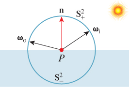
Figure 27.1: We’ll consider a surface (shown shaded) with normal vector n; ![]() consists of all vectors pointing away from the surface, while
consists of all vectors pointing away from the surface, while ![]() consists of vectors pointing into the surface. Light arrives from a source that’s in direction ω
consists of vectors pointing into the surface. Light arrives from a source that’s in direction ω ![]()
![]() , and scatters in directions ωo, which may be in either
, and scatters in directions ωo, which may be in either ![]() or
or ![]() .
.
Before we describe the kinds of scattering, we caution that some terms are used very informally. For example, “diffuse” can be used to mean “anything except mirror reflection” or “very similar to Lambertian.”
Here is a collection of terms used for scattering, with figures showing some of them.
• Reflective (Figure 27.2): The scattered light is all in the upper hemisphere, that is, ωo · n ≥ 0. More precisely, fs(ωi, ωo) = 0 for ![]() .
.
• Transmissive (Figure 27.3): The scattered light is all in the lower hemisphere, that is, ωo · n ≤ 0. More precisely, fs(ωi, ωo) = 0 for ![]() .
.
• Mirror (Figure 27.4; “specular” is a synonym): The scattered light is all in a single direction, the mirror-reflection direction ωr = 2(ωi · n)n – ωi. The “function” fs has an infinity: fs(ωi, ωo) = ∞. More precisely, trying to measure the reflectance in the usual way fails, because the outgoing radiance is independent of the solid angle subtended by the light source; this means that our usual BSDF approach is inappropriate for handling mirror-reflected light.1 Practically speaking, this means that in the programs you write, you need to handle mirror reflection as a special case.
1. ![]() In truth, this is a case where the notion of “distribution” applies: What we tend to write as integrals involving the BSDF typically have the form ∫ fsLg, where L is some representation of radiance and g represents other terms like change of variables Jacobians, etc.; such integrals transform the radiance field L into either a number or another function, and they do so linearly. Thus, “integrating against the BSDF” is just a way to write a linear function from one function space to another. A few such linear maps cannot be written this way, just like the “delta functions” of Chapter 18, but in the quest for consistent notation, researchers in graphics pretend that they can and claim the BSDF “is infinite” at certain points of its domain.
In truth, this is a case where the notion of “distribution” applies: What we tend to write as integrals involving the BSDF typically have the form ∫ fsLg, where L is some representation of radiance and g represents other terms like change of variables Jacobians, etc.; such integrals transform the radiance field L into either a number or another function, and they do so linearly. Thus, “integrating against the BSDF” is just a way to write a linear function from one function space to another. A few such linear maps cannot be written this way, just like the “delta functions” of Chapter 18, but in the quest for consistent notation, researchers in graphics pretend that they can and claim the BSDF “is infinite” at certain points of its domain.
• Impulse: The scattered light is all in a single direction, but this direction is not necessarily the direction of mirror reflection. For example, we may want to model a camera lens as purely transmissive, with all light transmitted according to Snell’s law. Once again, such impulse cases require special handling in our programs.
• Glossy (Figure 27.5): The scattered light is concentrated around some particular direction ωs ![]()
![]() , which is typically at or near the mirror-reflection direction. As noted earlier, the word “specular” is sometimes used to mean “glossy,” typically when the concentration of scattered light is very tight. The reflection from an enameled coffee mug has a substantial glossy component: You can see things reflected in the mug’s surface, although they appear slightly blurred. A waxed linoleum floor has a somewhat glossy appearance: You may be able to see objects reflected in it, but usually you can only see the gross outlines, and all detail in the reflection has been blurred away. The concentration of the scattered light is much less than that scattered from the enameled mug. The Phong model of Chapter 6 is a glossy-scattering model.
, which is typically at or near the mirror-reflection direction. As noted earlier, the word “specular” is sometimes used to mean “glossy,” typically when the concentration of scattered light is very tight. The reflection from an enameled coffee mug has a substantial glossy component: You can see things reflected in the mug’s surface, although they appear slightly blurred. A waxed linoleum floor has a somewhat glossy appearance: You may be able to see objects reflected in it, but usually you can only see the gross outlines, and all detail in the reflection has been blurred away. The concentration of the scattered light is much less than that scattered from the enameled mug. The Phong model of Chapter 6 is a glossy-scattering model.
• Diffuse: The scattered light is spread out in all possible directions, that is, f (ωi, ωo) is nonzero for all ωo ![]()
![]() , or, more weakly, f (ωi, ωo) > 0 for a large fraction of all directions. Many of the materials we encounter in everyday life exhibit diffuse scattering: paper, wood, brick, most cloth, etc.
, or, more weakly, f (ωi, ωo) > 0 for a large fraction of all directions. Many of the materials we encounter in everyday life exhibit diffuse scattering: paper, wood, brick, most cloth, etc.
• Lambertian (Figure 27.6): This is a special case of diffuse reflection in which the outgoing radiance in direction ωo is independent of ωo. No matter what position you view it from, a diffuse surface looks equally bright. This means that the BRDF, as a function of its second argument, is constant: ![]() for any two vectors ωo,
for any two vectors ωo, ![]() .
.
• Retroreflective: A surface is retroreflective if fs(ωi, ωo) is relatively large for some vector ωo that’s close to ωi. Often the surface is specular, and the specular peak direction is very near ωi. Retroreflective paint is used on road signs to make them more visible to drivers (whose headlights illuminate the signs), and retroreflective fabrics are often sewn into clothing for athletes to make them particularly visible to cars at night.
• Refractive: This is a special case of transmission analogous to mirror reflection: The transmitted light all lies in the direction ωt ![]()
![]() determined by Snell’s law.
determined by Snell’s law.
For each of the classes of scattering described above, we can translate the description into a characterization of the BSDF, with some of the characterizations more precise than others. Because the BSDF is a function of two arguments, the direction ωi of the arriving light and the direction ωo of the scattered light, it’s difficult to give a complete depiction. Instead, we pick a representative direction ωi, and we plot the BSDF as a function of ωo, that is, we draw a representation of the function ωo ![]() fs(ωi, ωo). We further simplify by limiting ourselves to the case where ωi, n, and ωo are all in the same plane; with this restriction we can draw a radial graph in the plane as shown in Figure 27.7.
fs(ωi, ωo). We further simplify by limiting ourselves to the case where ωi, n, and ωo are all in the same plane; with this restriction we can draw a radial graph in the plane as shown in Figure 27.7.
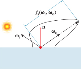
Figure 27.7: Plotting the BSDF. The arriving light comes from the left along direction –ωi; a typical outgoing direction ωo is shown. The polar plot intersects the radial direction of ωo at a distance fs(ωi, ωo).
The dependence of the BSDF-curve shape on ωi tends to be relatively simple in many cases, so this single plot can give a good sense of the overall function.
One important thing to understand is that the BSDF curve is not the pattern of emitted radiation. You might imagine that if you sent a stream of photons toward the material traveling in direction –ωi, the resultant outgoing photons (e.g., in the ωi – n plane) would have an angular distribution given by the BSDF curve in that plane (i.e., where the BSDF curve is twice as large, the probability density of a photon emerging in that direction is twice as large). That’s not correct, however, as we can see by considering a perfect Lambertian reflector, for which fs(ωi, ωo) = 1/π for all ωi, ωo ![]()
![]() . (We’ll soon see why 1/π is the right constant.)
. (We’ll soon see why 1/π is the right constant.)
Suppose for a moment that for a photon arriving from a source in direction ωi, the probability density of scattering in direction ωo were the same in all directions ωo. To estimate the radiance at a point Q1 on the unit hemisphere around some surface point P (see Figure 27.8), we’d take a solid angle Ω1 at Q1 and measure the density of the light energy arriving in that solid angle. For the radiance to be constant, as we know it is for a Lambertian surface, we’d have to get the same value when we estimated it at Q2 with a solid angle Ω2 of the same measure. But the amount of reflecting surface subtended by the two solid angles varies like the inverse of the “outgoing cosine,” leading to an extra 1/(ωo · n) factor in the outgoing radiance. The probability density of an incoming photon being scattered in direction ωo from a Lambertian surface must therefore be proportional to fs(ωi, ωo)(ωo · n).
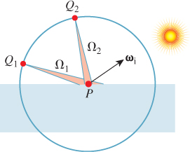
Figure 27.8: Computing the radiance at points near a hypothetical surface from which photons scatter equally in all directions.
Figure 27.9 shows several overlapping classes of scattering that we’ve discussed, with the BSDF drawn in black and the scattering probability density drawn in blue.
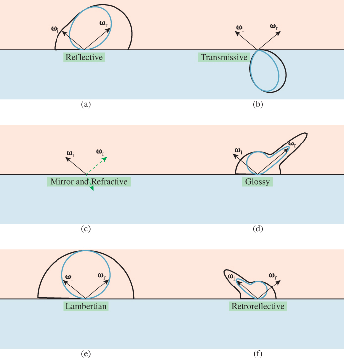
Figure 27.9: BSDF (black outer curves) and probability density plots (blue inner curves) for several classes of reflections; for impulse scattering, like mirror reflection, we’ve indicated the impulse direction with a green arrow as in the two right-pointing arrows in (c). For the others, the peaks in probability density and BSDF are offset from one another because of the cosine weighting. (a) A generic reflective material. (b) A purely transmissive material, which is physically unrealistic. (c) A material with mirror and refractive impulses; this is the kind of scattering we expect at an air-to-water interface. (d) Glossy scattering. (e) Lambertian scattering. (f) Retroreflective scattering.
27.5. Empirical and Phenomenological Models for Scattering
We now introduce a few basic scattering models that will serve several functions. The mirror and Lambertian models are the basis for several microfacet-based models that we’ll discuss when we examine physically based models. And the Blinn-Phong model, although not strictly physically based, is very widely used in practice.
27.5.1. Mirror “Scattering”
An ideal mirror-reflecting plane (for which all light is reflected rather than absorbed), shown in Figure 27.10, reflects light from a source in such a way that the emitted light distribution is exactly the same as would be produced by an identical source at some position behind the mirror’s location (assuming the mirror was removed). Because the outgoing radiance along each ray in these two situations is the same, the mirror-reflection process evidently results in no change in the net light energy in the scene.
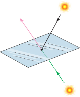
Figure 27.10: A mirrored plane, reflecting a light source above the plane (black solid line), produces the same outgoing radiance field (pink) as a “virtual” source below the plane placed at the proper location behind the mirror would produce (dashed green) in the absence of the mirror.
Perfect mirrors are rare. More commonplace is that a mirrored surface in fact absorbs some amount of light, and reflects the remainder. The outgoing radiance along the mirror direction ωr = ωi – 2(n · ωi)n is therefore a constant multiple of the incoming radiance:
where the reflectivity ρ is a number between 0 and 1. All that’s needed to specify the mirror reflectance from a surface is the normal vector n and the reflectance constant ρ, which is unitless. This constant may, however, have some spectral dependence (i.e., light at different wavelengths may be reflected differently).
The spectral dependence of reflectance depends on the underlying material. In broad terms, for insulators like plastic, the mirror-reflected light has the same spectral distribution as the incoming light, while for conductors, certain frequencies of light are preferentially reflected. This is why a polished piece of plastic has white highlights, while a polished piece of gold has gold-colored highlights. We’ll return to this in Section 27.8.3.
The simplest summary representation of the spectral dependence of the reflected light is to just give RGB values, representing the overall reflectance of the material in response to long-, middle-, and short-wave incoming radiation. Thus, the summary computational model becomes
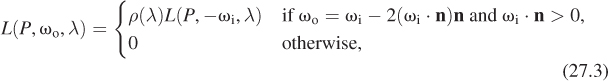
where λ represents the wavelength of the light as usual.
This simple model of mirror reflection ignores the Fresnel equations that arise from the polarization of light. There is no physical surface that actually reflects like a perfect mirror (or one with constant reflectivity 0 < ρ < 1) for all angles of incoming and outgoing light. We’ll return to a more sophisticated version of mirror scattering when we discuss physically based models.
27.5.2. Lambertian Reflectors
A Lambertian surface has the property that when it’s illuminated, the outgoing radiance in every (reflected) direction is the same (there’s no transmission). Furthermore, this outgoing radiance varies linearly with irradiance: Whether we reduce the incoming illumination or make it arrive at a grazing angle, the outgoing radiance varies in the same way. Thus, the BRDF is constant; we usually write fs(P, ωi, ωo) = ρ/π, where ρ is a constant indicating what fraction of the arriving light energy is scattered.
Let’s now check for which values of ρ this reflector will be energy-conserving. Imagine (as shown in Figure 27.11) that light arrives at a small, rectangular region, R, of material with area A, from a source like the sun: All incoming rays are in some small, solid angle Ω, and the radiance along each ray in a direction from Ω is the same constant ![]() . Then the total rate of energy arrival at the surface region R is the integral over R and Ω of the arriving radiance, multiplied by the dot product of the incoming direction and surface normal:
. Then the total rate of energy arrival at the surface region R is the integral over R and Ω of the arriving radiance, multiplied by the dot product of the incoming direction and surface normal:
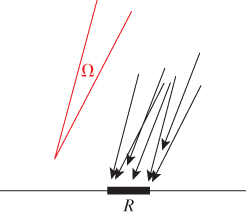
Figure 27.11: Light arrives at a small, rectangular sample R from directions ω ![]() Ω, a small solid angle; the radiance of the incoming light is independent of position and angle.
Ω, a small solid angle; the radiance of the incoming light is independent of position and angle.
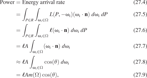
where m(Ω) denotes the measure of the solid angle Ω, and θ is the angle between a typical vector ω ![]() Ω and the (constant) surface normal n. As Ω gets small, the approximation of the dot product by a single central dot product gets increasingly accurate.
Ω and the (constant) surface normal n. As Ω gets small, the approximation of the dot product by a single central dot product gets increasingly accurate.
Use the reflectance equation to show that the radiance of a ray emitted from the region R is well approximated by![]() (ρ/π) cos(θ)m(Ω).
(ρ/π) cos(θ)m(Ω).
To compute the rate at which light energy is emitted, let us surround the sample by a very large, black, completely absorptive hemisphere, and determine the rate of energy arrival at that sphere. Just as in Chapter 26, we’ll make the sphere so large that the ray from the point Q to any point on the emitter R always has essentially the same direction, independent of the emitter point.
The density d(Q) of light energy (per second) arriving at a point Q of the hemisphere is the integral, over all directions, of the radiance arriving at Q. Since the only source of incoming light is the region R, this simplifies to an integral over directions ω that point from Q to some location in R; we’ll denote this set of directions ΩQ. The density is then
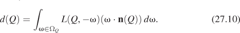
We know the radiance arriving at Q from the inline exercise above. Furthermore, since the disk R appears very small as viewed from Q, the vectors ω all point in approximately the same direction (namely, S(P – Q), where P is the center of the region R, and hence the center of the sphere as well). This means that we can approximate d(Q) well by
The last dot product is approximately 1, because ω points almost exactly toward the center of the large sphere on which Q lies. We can rewrite the measure of ΩQ as (A/r2) cos(θ′), where θ′ is the angle between n and Q – P, that is, the outgoing angle, to get
Everything in this expression is constant (as a function of Q) except the final cosine. When we integrate this power density over the entire hemisphere, to get the total power arriving at the hemisphere, the result is
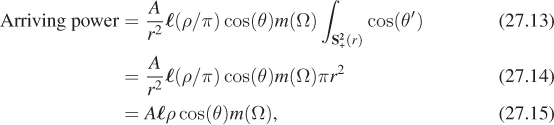
which is exactly ρ times the power that arrived at our Lambertian surface. So the scattering conserves power only if ρ ≤ 1.
The computational model for a Lambertian surface consists of a normal vector and a per-wavelength (or per-primary) reflectance value.
The number ρ is called the Lambertian reflectance value; it also happens to be the cosine-weighted integral of the Lambertian BRDF over the upper hemisphere, and it represents the fraction of arriving power that’s reflected by the surface. While such a notion might be useful for other kinds of scattering as well, for a general BRDF fr the ratio of leaving power to arriving power depends on the distribution of arriving power, so reflectance becomes a function of both the BRDF and the light field. We’ll have no use for this more general notion.
As a final observation about Lambertian surfaces, we note that the argument above describing the difference between the BRDF and the probability of photon scattering tells us that if a photon arrives at an ideal, perfectly reflecting (ρ = 1) Lambertian surface traveling in direction –ωi, it leaves in some other direction ωo, which can be thought of as being drawn from some probability distribution with probability density function p. The distribution p is given by
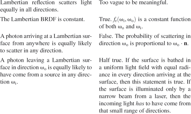
Here are a few common statements about Lambertian reflection, with commentary.
27.5.3. The Phong and Blinn-Phong Models
You’ve already seen two forms of the Phong model: the first in Chapter 6, where light was measured in some ill-defined units of “intensity,” with values ranging from 0 to 1, and the second in Section 14.9.3, where actual physical units were used, and the constants had been adjusted so that the model was energy-conservative provided that the sum of the specular and diffuse constants was no greater than 1. In addition, the latter form eliminated the so-called “ambient” term, which was an ad hoc construct that was included to simulate the effects of multi-bounce light transport in a scene.
The general form of the simplified Blinn-Phong BRDF from Chapter 14 is given by

In Equation 27.17, h is called the half-vector and kL and kG are the Lambertian and glossy reflectances, respectively, and may range from 0 to 1. The model is energy-conservative if kL + kG ≤ 1.
Blinn’s actual model was derived from physical considerations motivated by the microfacet models we’ll discuss shortly, and also included a factor for the Fresnel equations, but we’ll omit those details for now.
27.5.3.1. Historical Notes
The original Phong model described the reflected light in terms of “intensity,” which was not carefully defined, and included a third term, for reflection of “ambient light,” that is, all the light in the scene that underwent multiple reflections until it was widely diffused. Thus, you’ll sometimes encounter reflection models that use an ambient, a diffuse, and a specular reflection constant, as you saw in Chapter 6.
Phong’s original model also had just one constant for the specular term (which we call the glossy term); this meant that reflectance was independent of wavelength, and a white directional light tended to produce a white highlight, no matter what the material. This wavelength independence is characteristic of many insulators, but does not hold for conductors in general (e.g., look at the reflection of a white light in a gold ring). The specular reflectance was therefore given a wavelength dependence (typically by specifying red, green, and blue reflectance values). The diffuse reflectance was similarly extended to include RGB variation (e.g., a red shirt reflects lots of red light, and little blue or green light). And finally, the intensity of light was known to fall off quadratically as a function of distance from the light source (although this notion was problematic for “directional light sources” that were assumed to be “at infinity”!). Thus, for many years the “standard” lighting model looked like
where the terms labeled I are all “intensities,” the k factors are the constants associated with ambient, diffuse, and specular reflection (we’ve folded the ambient, diffuse, and specular “color” into these for simplicity), h is the average of the vector to the light and the vector to the eye, ns is the specular exponent, d is the distance from the light to the point P, and
was a “quadratic falloff” term, although in practice c was often set to zero, and there’s no reasonable explanation for the “min” in the expression except that “things got dark too fast otherwise.” When there were multiple light sources, the bracketed term in Equation 27.20 was repeated once per source.
From a modern viewpoint, this entire model, especially the “ambient term,” was a terrible thing: Instead of solving the underlying problem (light transport), you apply a “hack” in a completely different area (scattering at a point). But from the point of view of the engineering of the day, it was a reasonable choice: Doing accurate light-transport computations was clearly beyond the capacity of the computers of the day, while evaluating the more straightforward solution provided by Phong’s model was relatively simple and drastically improved the empirical results. But you should not be fooled into thinking that the model has any physical basis.
There’s also a terminology challenge: The computation of the amount of light reflected from a surface was sometimes called “lighting” or “illumination,” although the standard interpretation of these words as descriptions of the light arriving at the surface was also common. The “lighting model” was typically evaluated at the vertices of a triangular mesh and then interpolated in some way to give values at points in the interior of the triangle. This latter interpolation process was known as shading, and you’ll sometimes read of Gouraud shading (barycentric interpolation of values at the vertices) or Phong shading, in which, rather than interpolating the values, the component parts were interpolated so that the normal vector was reestimated for each internal point of each triangle, and then the inner product with the incoming light vector was computed, etc. In each case, the desire was to reduce the artifacts arising from computing the scattering only at the triangle vertices. One of the problems, for instance, with Gouraud shading was that the different rates of intensity variation in two triangles that shared an edge led to an enhanced perception of that edge through Mach banding (see Sections 1.7 and 5.3.2) rather than causing the edges to disappear. Thus, although the quality of the approximation to the ideal was good when measured in physical terms (“How different is the intensity from the true one?”), in perceptual terms (“How different does this surface appear from the true surface?”) it was not.
Nowadays we refer to shading and lighting differently: The description of the outgoing light in response to the incoming light is called a reflection model or scattering model, and the program fragment that computes this is called a shader. Because of the highly parallel nature of most graphics processing, the scattering model is usually evaluated at every pixel, often multiple times, and the “shading” process (i.e., interpolation across triangles) is no longer necessary; furthermore, so many triangles are subpixel in size that this interpolation would never be used anyhow. So the modern use of the word “shader” is unlikely to lead to confusion.
27.5.4. The Lafortune Model
The Phong model expressed the specular component of the BRDF as a cosine power (specifically, as a power of the cosine of the angle between the outgoing direction and the mirror-reflection direction). Letting R(ω, n) denote the mirror-reflection direction of ω at a surface with normal n—in the case where n = [0 0 1]T, R(ω, n) is just [–ωx –ωy ωz]T—the glossy part of the Phong BRDF is simply
where C is a normalization constant. This BRDF is evidently reciprocal in the case where n = [0 0 1]T: Swapping ωo and ωi merely negates the x- and y-coordinates of each vector, thus leaving the dot product unchanged.
Why does the reciprocality in the case where n = [0 0 1]T prove that the formulation is reciprocal in all cases?
Lafortune et al. noticed that measured BRDFs tended to have lobes that were not necessarily centered about the mirror direction, and that sometimes they appeared to have multiple lobes. By taking a sum of Phong-like terms, but with varying substitutes for the mirror direction, they generalized to produce a much richer model, based on a collection of lobes centered at k different vectors {ωk : k = 1, . . ., n},
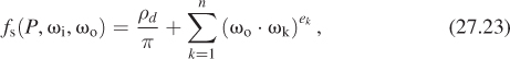
where ρd is the diffuse reflectivity. For this to be reciprocal requires that the vectors ωk be expressed as term-by-term multiples of ωi so that ω1, for instance, is
Alternatively, one can express this by building a diagonal matrix A1, and then saying that ωk = A1ωi. Then the Lafortune model ends up being
where the fact that the matrices Ak are all diagonal guarantees that the BRDF is reciprocal.
Quickly verify the preceding claim. Now suppose that A1, instead of being diagonal, represents rotation through 90° about the z-axis. Show that the resultant BRDF is not reciprocal. Conclude that the Lafortune BRDF is reciprocal if and only if all the matrices Ak are symmetric.
In practice, since the Lafortune model only uses diagonal matrices, it makes much more sense to just store the three diagonal entries than the whole matrix, and to treat the matrix-vector multiplication as a term-by-term multiplication.
The Lafortune model is very general. In fact, it’s possible to approximate almost any conservative, reciprocal function on S2 × S2 by using a large enough value of n. But to get a good fit may require a very large n indeed.
To add spectral dependence to the BRDF representation, we need to let the diagonal matrices Ak (or their three diagonal entries) be functions of wavelength; this is typically done with RGB values.
The Lafortune model is a hybrid. It’s based on a phenomenological model (Phong), but it is motivated by a rather different kind of phenomenon: the appearance of measured BRDFs! In some sense, the Lafortune model can be seen not as a model of light scattering, but as a model of a class of functions, with the property that observed BRDFs tend to be representable with relatively few coefficients, and hence be amenable to rapid evaluation.
27.5.5. Sampling
We’ve described the BRDF for the mirror and Lambertian and Blinn-Phong models in a form where, given ωi and ωo, you could easily compute fs(ωi, ωo). But in ray tracing/path tracing and photon mapping, which we’ll describe in more detail in Chapters 31 and 32, there are two other computations we need to perform.
For photon mapping, we’re given ωi and we need to randomly select a vector ωo with probability density proportional to fs(ωi, ωo)(ωo· n). (Probability densities are described in detail in Chapter 30; for now it’s sufficient to think, “We want to pick a vector ωo more often if fs(ωi, ωo)(ωo · n) is large, and less often if it’s small.”)
For mirror reflection, this is easy: We always return ωr, the mirror-reflected version of ωi. For Lambertian scattering, we need to pick a direction on the hemisphere, favoring the North Pole, and fading off in probability as we approach the equator. Fortunately, using the Average Height principle, it’s not too difficult to do this. Section 30.3.8 gives the details.
For Blinn-Phong scattering, things are not so simple. Although it’s possible to sample directly from the BRDF by doing some careful computations, that’s only because of the nice power-of-a-cosine form; by the time other factors, like the Fresnel term, get included such direct sampling is no longer possible. Far better is to use an approach like that of Lawrence [Law04], which approximates the BRDF with terms that are amenable to efficient sampling.
For ray tracing/path tracing, we have a similar problem, except that we’re given ωo and want to select ωi with density proportional to fs(ωi, ωo). And for direct computation of the reflectance integral, we may want to sample in proportion to fs(ωi, ωo)(ωi · n).
The same arguments apply in these cases, except that in the Lambertian case for the ray tracing/path tracing computation, instead of using the cosine-weighted BRDF, we just need to sample in proportion to the BRDF, which is constant. In other words, we just need to pick points uniformly on the hemisphere, which is easy with the cylinder-sphere projection theorem.
27.6. Measured Models
Phenomenological models tend to approximate well those things that we, as humans, recognize as “phenomena.” But it’s possible that other aspects of scattering, when combined with light transport, produce other “phenomena” as well, and if we suppress those aspects, these secondary phenomena will never be simulated. The only way to know is to have a ground-truth representation of the scattering, and compare results of simulations that use this ground truth to those that use either phenomenological or physically based approximations to it, and see whether the results differ significantly.
One such ground-truth representation is provided by the full BRDF measurements made by Matusik et al. [MPBM03] of about one hundred isotropic materials. For an isotropic material, the BRDF, represented in polar coordinates, depends only on the difference between the longitude coordinates of ωi and ωo, so the data can be tabulated in a three-index table (two latitudes, one longitude difference). Tabulated at approximately one sample per degree, these tables have many entries (90 × 90 × 180), each of which is an RGB triple. (The sampling near glossy highlights is deliberately somewhat denser so that very shiny materials can be accurately represented.)
Others have measured various anisotropic materials [War92], texture characteristics of surfaces [DvGNK99], and more complex data like subsurface scattering distribution [JMLH01], and have developed image-based approaches to measuring BRDFs without the high cost of a gonioreflectomer [MLW+99].
One value of these measurements is that they can be used to compare the expressive power of various BRDF models: if optimally adjusting all the parameters of the Blinn-Phong model, for instance, only allowed you to get within 5% of the measured values, and that only for, say, 90% of all possible (ωi, ωo) pairs, you might conclude that the Blinn-Phong model was not sufficiently rich to represent real materials decently. Matusik in fact took this approach in comparing two BRDF models, the first due to Ward [War92] and the second to Lafortune [LFTG97]; he found that the Lafortune model was better able to fit the data in many cases, but even so, there were cases for which the average error was as large as 20%, where the difference was measured as a difference of logarithms, to discount somewhat the overwhelming effect of glossy peaks in the BRDF.
One drawback to using measured BRDFs in rendering is the cost of performing effective sampling. While Matusik describes techniques for this, they require a large amount of extra precomputed data and are still slow compared to those few models for which explicit sampling techniques are known.
There are some limits to using measured BRDFs. We can only render images of scenes for which we know the BRDFs of all materials, and measuring the BRDF of a material is nontrivial; gathering observations at grazing angles is particularly challenging. And we can only gather the BRDF of a material that already exists. We can’t create new BRDFs by adjusting parameters, as we can do with the various physically based models described below. Finally, there’s the problem that the gathered data may well contain errors, errors that can make the observed BRDF turn out to be physically unrealistic. Matusik handles this in part by projecting every measured BRDF onto the reciprocal-BRDF subspace, by replacing fs(ωi, ωo) with the average of fs(ωi, ωo) and fs(ωo, ωi), thus ensuring reciprocity, and by discarding certain outlying measurements.
27.7. Physical Models for Specular and Diffuse Reflection
We now turn to physically based models of reflective scattering. There is a choice to be made in attempting to explain scattering phenomena: Should we use physical optics, based on the wave theory of light, in conjunction with a geometric model, to determine the scattering, or geometric optics, in which the reflection of light by surfaces is determined entirely by a billiard-ball-bounce model, in which the arriving light reflects from the surface in the mirror direction? At first glance, the geometric optics approach seems destined for failure; after all, not every surface is mirrorlike. This can, however, be addressed by examining the interaction of light with a rough surface, in which the reflection is mirrorlike, but the geometry is extremely complex, consisting of many tiny reflecting facets oriented in many possible directions. Since the roughness can be described probabilistically, this approach is actually feasible. In contrast, the physical optics approach presents enormous computational challenges, in the sense that to apply it, we must apply Maxwell’s equations to relatively complex situations, where any hope of an easily expressed formula is lost; our best hope is for rapid numerical solutions of the equations. We’ll return to this after examining the geometric optics approaches.
Geometric optics is really only appropriate when the small reflecting parts of the surface are large compared to the wavelength of the incident light. Since the incident light that interests us is in the visible range, we can say that the wavelength is about 0.5 to 1.0 microns; this means that the microfacets must be at the very least 1 micron in size. When you recall that a human hair is on the order of 15 microns in diameter, and that it’s easy to feel a single hair on a flat surface, you realize that the geometric optics assumption for ordinary materials is just barely reasonable: 15 micron sandpaper feels about like newsprint; 2 micron sandpaper is used to smooth out automotive finishes and to polish sharp knives. Thus, materials whose roughness is between that of a highly polished metal and a piece of newsprint are likely to contain scratches that are on the scale of a few wavelengths of light. Despite this, the geometric optics approach seems to make good predictions in practice at this scale. We’ll describe the main ideas of the geometric optics approach in the next several sections.
We do so with a caution, however: Given the scale disagreements (facets must be large compared to the wavelength of light, but in practice are quite close to it), these models are at best weak approximations of the underlying phenomena. Recent careful measurement work has shown the weakness of the approximations [Lei10].
27.8. Physically Based Scattering Models
The underlying physics of reflection from a flat surface depend on the electrical properties of the atomic structure of the material, some of which we described in Chapter 26. In particular, metals, which tend to make the best mirror reflectors, have many free electrons that float about the surface, creating an almost perfectly planar sheet of constant electrical potential with which the electromagnetic light-wave interacts. The Fresnel equations determine the degree of reflection for light of varying polarizations; in graphics, we typically assume unpolarized light, and thus average the perpendicular and parallel terms of the Fresnel equations. We’ll review these equations, and describe how they’re applied in practice, since they are part of all the physically based scattering models.
As we said, the assumption, in the physical computations that support these reflectance models, is that the reflecting surface is large compared to the wavelength of the arriving light, or else diffraction will start to dominate. The mirror-plane model can also be used to compute the reflection from a mirror surface that’s nonplanar, provided that its curvature is not too great; to compute the reflection at a point Q, we use the normal vector n(Q) to compute the mirror direction just as before. If the curvature is too large (i.e., if the normal vector changes too fast), then again the “sheet of constant potential” model fails, and diffraction starts to dominate. A radius of curvature (in any surface direction) that’s near or lower than the wavelength indicates a place where the mirror model is no longer appropriate. It’s worth noting that in polygonal models, the curvature at every point of every edge is infinite. This is typically ignored in ray tracers, where a ray hits either one facet or the other, and proximity of the ray to an edge is ignored. If the ray actually hits an edge precisely, it may be ignored or treated as lying on one of the two adjacent surfaces. The results look correct enough that they have not generally been a point of concern.
27.8.1. The Fresnel Equations, Revisited
In Chapter 26, we saw that at a surface between dielectric materials such as water and air, or glass and air, the amount of light reflected and transmitted depended strongly on the angle of the arriving light. Under the assumption that the arriving light was unpolarized, the fraction of light energy reflected is a function of the refractive indices of the two materials and the incident angle θi = cos–1(ωi · n), and the angle of the transmitted ray is θt. The Fresnel reflectance RF is the average of the parallel- and perpendicular-polarized terms, Rs and Rp, which are given by
Recall that θi and θt are related by Snell’s law:
For an air-water interface, we have n1, the refractive index of air, is approximately 1.0, while that of water is approximately 1.33. The plot of RF as a function of θi is shown in Figure 27.12.
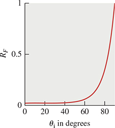
As you’ll observe, the function is nearly constant until we approach grazing, at which point it rises rapidly. If you plot FR for some other ratios of refractive indices (see Exercise 27.5), you’ll see that this characterization is quite general: nearly constant for small angles, a sudden rise near grazing angles.
For metallic surfaces, the formula for RF is somewhat more complex, but it exhibits the same general characteristics.
Schlick [SCH94] observed that for metallic surfaces RF could be well approximated by a simple expression, and others have observed that the approximation works reasonably well even for nonmetallic materials. The approximation is
where RF(0) is the reflection at normal incidence (θi = 0) and θi = cos–1(ωi · n) is the angle of incidence. When the cosine is 1, we get RF(0); when the cosine is 0, we get 1.0.
There’s usually no reason to compute θ explicitly, since many formulas involve the cosine or sine of θ rather than θ itself. Rewrite Schlick’s approximation in terms of ωi and n rather than θ.
For insulators, RF(0) tends to be small, so there’s large variation in RF with angle θi, leading to a pronounced Fresnel effect. For conductors, RF(0) tends to be large (typically greater than 0.5), so the Fresnel effect is less pronounced.
Note that the index of refraction and the coefficient of extinction depend on wavelength (although they have not been tabulated for many materials, which is a problem); this means that the Fresnel reflectance is also a function of wavelength. For many metals, this dependence is considerable. For gold, for instance, the extinction coefficient drops substantially above about 500 nm, while the index of refraction rises steadily above about 500 nm, which together give gold its characteristic yellow appearance. For insulators, the refractive index is nearly constant with respect to frequency, causing highlights on insulators to be the color of the incoming light.
Actually using the Schlick approximation requires that you know RF(0). But the original Fresnel equations (for dielectrics) give you this value:
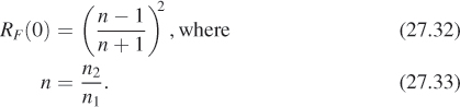
In graphics, most objects sit in air, so n1 = 1, and the formula is slightly simpler: You just replace n with n2.
Show that in the case of conductors, the correct form is
using the approximation of the Fresnel reflectance for conductors.
We sometimes want to render things like an underwater view of the surface of a swimming pool. In this case, the light rays are traveling in a medium of large refractive index, and the “other” side is air, which has lower refractive index. Of course, Fresnel’s equations still hold, as does the Schlick approximation, but to make it work you must use θt, the angle of the transmitted ray (the one in the air, not the water) as the argument. The result is that the Fresnel reflectance approaches 1.0 as θi approaches the critical angle, which is generally much less than 90°. (For angles greater than the critical angle, RF remains at 1.0.)
If you have looked up at the pool’s surface while swimming, explain the appearance of the surface from below, and the difference in its appearance from above, by considering the Fresnel reflectance and the critical angle for total internal reflection.
27.8.2. The Torrance-Sparrow Model
The Phong model predicts that a surface illuminated in direction ωi will reflect light in all directions, with a peak in the mirror-reflection direction ωr. In actual observations of nonmirror materials, that’s not the peak direction. Torrance and Sparrow provided a model to explain this off-mirror peak: They imagined that the surface was made up of microfacets, each of which was a tiny mirror reflector, but with random orientations. The microfacets were assumed to pair up to form “V” shapes, with identical slopes of each side of the “V” so that an edge-on slice of the material appeared as a collection of grooves of varying depth, all with their tops at the same height, as in Figure 27.13.
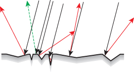
Figure 27.13: The symmetric grooves all have their tops at the same height. Light arriving at an angle (downward-pointing black arrows) can be reflected in the mirror direction (the dashed green arrow), or reflect back toward the source or in other directions (red).
Note that we are implicitly assuming that the BRDF we’re estimating is for a measurement area that’s substantially larger than the scale of a single microfacet, or the analysis, which is based on average microfacets, is no longer reasonable. For the same reason, when we use a measured BRDF in rendering it’s important that an imager pixel correspond to a surface region whose area is as large or larger than the area used in gathering the BRDF in the first place.
The wavelength of visible light is between one-half and one micron; it’s convenient to treat it as about one micron for back-of-the-envelope estimation. To prevent diffraction effects from being significant, microfacets should be at least a couple of wavelengths (say, five) in their minimum dimension. In a surface that’s fairly flat (most microfacets have slope less than 45°), we can imagine each microfacet is a small disk or square, so its projected length, in any direction, is at least .71 ≈ cos(45°) times its minimum dimension.
(a) Approximately how many such microfacets can fit into a 1 mm-diameter disk?
(b) If you had that many small mirrorlike facets in such a disk and illuminated them with a laser pointer whose beam covered just that disk, what would the pattern of reflected light look like? Get a laser pointer, a piece of polished metal, and a piece of white paper to “catch” the outgoing light and see whether the reflected light follows the predicted pattern.
For illumination arriving along the normal direction (ωi = n), the scattered light goes in many directions: If the grooves are all shallow, most of it reflects back in the normal direction; if they’re deep, there’s much more scattering in off-normal directions. But for illumination arriving in an off-normal direction, multiple phenomena combine to generate the scattering pattern.
• Each peak “shadows” the next valley to some degree, so the amount of light reflected from a microfacet is no longer proportional to its area.
• The reflected light may hit yet another microfacet, and be further reflected, and thus not continue in the reflected direction; this is called masking.
• For certain illumination directions, we can get both masking and shadowing, as shown in Figure 27.14.
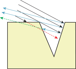
Figure 27.14: Incoming light misses the bottom part of the right-hand side of the V groove, which is shadowed (right-pointing red dashed ray); some of the light reflected from that right-hand side is masked by the left-hand side (left-pointing green dashed ray). (Courtesy of Ephraim Sparrow, “Theory for Off-Specular Reflection from Roughened Surfaces” by K. Torrance and E.M. Sparrow. It was printed in Journal of the Optical Society of America, Vol. 57, No 9, 1105–1114, September 1967. Redrawn.)
The detailed analysis of the effects of masking and shadowing, for various distributions of microfacet orientations, is quite complex [TS67], but the analysis predicts three important phenomena: The first is backscattering, in which some incoming light from off-normal directions is reflected back toward the source; the second is the off-specular peak—the peak value of the BRDF occurs not at the mirror-reflection direction, but at a more-grazing (i.e., less normal) direction. The third is that the value of the BRDF at grazing angles remains finite, which is in accord with experimental observation, but not with prior microfacet models that didn’t account for masking and shadowing.
By the way, it’s worth experimenting with a piece of ordinary office paper to see how very specular are the near-grazing-angle reflections from a supposedly matte surface. If in front of your face you hold a piece of paper by its bottom edge so that the top falls down, forming a “hill” that you can look across, and then you look at some fairly bright scene (the view out an office window on a sunny day works well), you can see quite distinct features reflected in the paper at or near the silhouette edge.
The Torrance-Sparrow model, like the Phong model, combines a diffuse term with the glossy term, and takes into account the Fresnel equations in adjusting the reflectivity as a function of incoming-light angle. The distribution of microfacet slopes is assumed to be exponential: The probability density at slope α is proportional to exp(–c2α2), where the constant c is a parameter of the model.
The parameters for the model are the index of refraction (which is wavelength-dependent), the slope-distribution constant c, and the diffuse and glossy constants kd and kg, although they use the ratio g = kg/kd as well, using a complex-number version of the index of refraction to represent both the ordinary index of refraction and the absorption. Torrance and Sparrow report that c = 0.05 works well, and approximately agrees with experimental observations of c = 0.035 and c = 0.046 for ground glass surfaces. They plot the predicted results for aluminum and magnesium oxide, and show good agreement with the observed data.
27.8.3. The Cook-Torrance Model
Cook and Torrance [CT82] developed an extension of the Torrance-Sparrow model that explicitly took into account the different nature of diffuse reflection (usually involving subsurface scattering, or multiple scattering from a sufficiently rough surface) and specular reflection, especially from metals, which is an almost entirely surface-based phenomenon. Since specular reflection from microfacets is again used to model glossy reflection, anything said about specular reflection here also applies to glossy reflection. The specular-diffuse difference means that the diffusely reflected and specularly reflected lights from a single surface may have quite different spectral distributions; plastics, for instance, tend to specularly reflect light with approximately the same spectral distribution as the illuminant, while metals (think of copper and gold) tend to have substantial spectral variation in reflectivity, so the reflected light “takes on the color of the material.”
As with the Phong model, there are three parts: an ambient, a diffuse, and a specular term. The ambient term is considered to be an average of the diffuse and specular effects due to light coming from many different directions in the scene, which is assumed to be uniform. Because of this, the color of the ambient term is a combination of the diffuse and specular colors (where we are using the term “color” as a shorthand for “spectral distribution”). The diffuse term is assumed Lambertian. The complete model, ignoring the ambient term, has the form
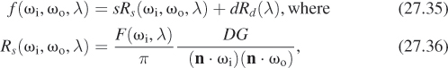
where s and d are the amounts of specular and diffuse reflectivity, respectively, Rs and Rd are the (spectral) BRDFs for specular and diffuse reflection, respectively, F is the Fresnel term, D is the microfacet slope distribution, and G is a geometric attenuation factor that accounts for masking and shadowing of facets; we’ve omitted the arguments for both D and G for now. The entire expression is evaluated at a point P of a surface with normal vector n(P), for which we’ll write n for simplicity.
It’s easiest to express the geometric term in terms of the half-vector
Using h, the geometric attenuation is
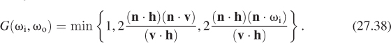
The slope distribution function D describes the fraction of facets that are oriented in each direction; letting α = cos–1(n · h), we can write D as a function of α, thus implicitly assuming that it’s symmetric around the surface normal, that is, that the microfacet distribution is isotropic. Cook and Torrance use the Beckmann distribution function
which has the single parameter m.
Convince yourself that if m is very small, then most facets are nearly perpendicular to the normal vector n, while if m is large, the surface is very rough with sharply angled facets.
They also note that a surface may be rough at several different scales; thus, the function D could be a weighted sum of multiple terms like the one in Equation 27.39.
Finally, they model the spectral distribution of the reflected light. For diffuse reflectance, they use measured reflectance spectra, which are typically measured with illumination at normal incidence; they note (as in our discussion of Fresnel reflectance above) that the diffuse reflectance spectra for most materials do not vary substantially for incidence angles up to 70° off normal, and even then vary relatively little. They therefore use the normal-incidence reflectance spectrum as the diffuse reflectance spectrum at all angles.
There are man-made materials that are designed to have reflectance spectra that vary with viewing angle; one example is a diffraction grating. Try to think of a diffuse material with this property. Hint: textiles.
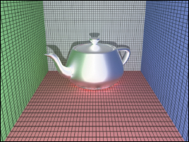
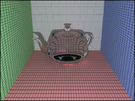
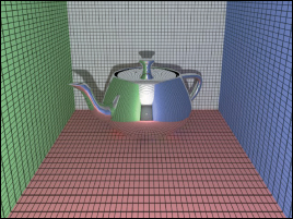
For the specular term, they model the angle dependence of the reflectance spectrum as coming entirely from the Fresnel term, as above. The results represented a huge step forward in computer graphics: Because the color of the specular highlights could now be different from that of either the underlying surface’s diffuse color or the color of the incident light, it became possible to plausibly simulate a much wider variety of materials (see Figure 27.15).
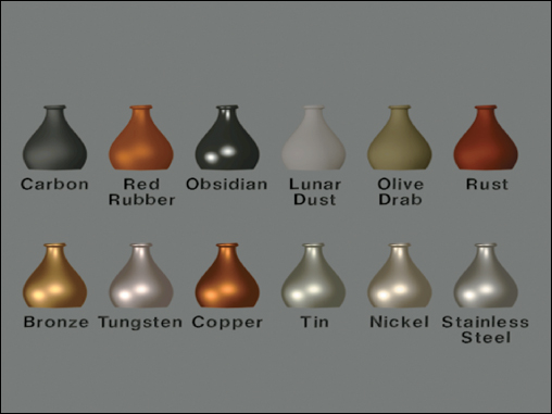
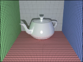
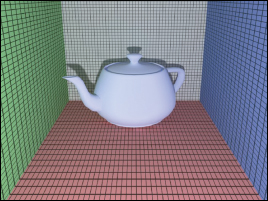
Figure 27.15: A single vase, illuminated by two lights, made of 12 different materials whose reflectance properties were determined with the Cook-Torrance model. (Courtesy of Robert Cook, ©1981 ACM, Inc. Reprinted by permission.)
27.8.4. The Oren-Nayar Model
Closely related to the microfacet models for specular reflection is the Oren-Nayar model [ON94] for reflection from rough surfaces such as unglazed clay pots, tennis balls, or the moon’s surface. Oren and Nayar observed that these diffuse reflectors did not actually follow Lambert’s law very well at all; in particular, the areas near the silhouette tended to be much lighter than Lambertian reflectance would predict. This is particularly obvious with the moon, whose brightness appears almost uniform across the surface (except for surface-texture features). They suggest that this brightness near the silhouettes can be explained by noting that the surface roughness means that even when we are looking near a silhouette, some parts of the surface are facing back toward us, and thus reflect more light than might be expected (see Figure 27.16). In particular, they apply essentially the Torrance-Sparrow-Cook idea of microfacets, but in a situation where they assume that each microfacet acts like a Lambertian reflector rather than a mirror.
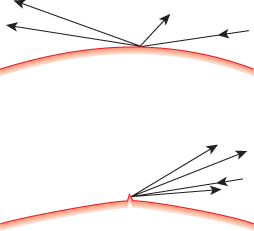
Figure 27.16: (Top) Near the edge of a smooth diffuse surface, very little light would be scattered back toward the viewer because the off-normal incidence of the light makes the irradiance small. (Bottom) If a small piece of surface near the silhouette is oriented more perpendicular to the incident light direction, this surface piece will scatter much more light in all directions, including the direction back toward the viewer.
Furthermore, they consider not only single-bounce interactions of illumination with microfacets, but multiple inter-reflections, observing that for a quite rough surface, illuminated at a nearly grazing angle and viewed from the opposite side from the illumination, each lighted facet is invisible to the viewer, but the facets that are not directly lit may nonetheless be visible. If you look east toward a mountain range at dawn, you cannot see the sunlight on the east sides of each mountain, but the west side of some mountains will be illuminated by light reflected from the east side of more westerly mountains (see Figure 27.17).
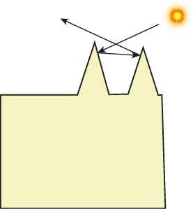
Figure 27.17: The west sides of mountains illuminated by the rising sun will be in shadow, but may be lit by light reflected from the east sides.
The expression for the radiance (assuming a Gaussian distribution of facet slopes) from a facet is a rather messy integral. Oren and Nayar evaluated this integral for many different directions of arriving light, viewer direction, and Gaussian shape parameters, and developed a much simplified form that’s suitable for more rapid computation of approximately correct values. The result is given in terms of θi, the angle between ωi and n, θo, the angle between ωo and n, and φ, the difference in azimuth between the incoming and outgoing light. If light arrives from the west and leaves to the east, then φ = 0; if it leaves to the northeast, then φ = 45°; if it leaves to the southeast, then φ = –45°, etc. The model has two parameters: the slope-distribution constant σ, where the probability of a facet at angle θ is proportional to ![]() , and the albedo, ρ, of the surface (which may be a function of wavelength).
, and the albedo, ρ, of the surface (which may be a function of wavelength).
The full-generality result is seldom used; instead, the simplified version, which accounts for only single scattering, is
and α = max(θi, θo) and β = min(θi, θo) and E0 is the irradiance.
27.8.5. Wave Theory Models
Until now, all of our models have used geometric optics, ignoring the effects of the wave nature of light (such as interference and diffraction), except for the Fresnel term. One reason for this is that working directly with Maxwell’s equations proves to be extremely difficult and computationally expensive. On the other hand, it does predict some effects that geometric optics models miss. The work of He [He93] makes the most compelling case for this, but the underlying physics is beyond the scope of this book; we refer the interested reader to the paper itself.
How important are wave effects? They certainly can matter, but as Pharr and Humphreys [PH10], p. 454, note:
Nayar, Ikeuchi, and Kanade [NKK91] have shown that some reflection models based on physical (wave) optics have substantially similar characteristics to those based on geometric optics. The geometric optics approximations don’t seem to cause too much error in practice, except on very smooth surfaces. This is a helpful result, giving experimental basis to the general belief that wave optics models aren’t usually worth their computational expense for computer graphics applications.
27.9. Representation Choices
A BSDF can be represented in various ways—as a table of values to be interpolated, as we saw for measured models, or as a sum of “lobes,” as in the Lafortune model, or even in a kind of “Fourier decomposition,” using spherical harmonics, which are the analog, on the 2-sphere, of the powers of sine and cosine on the circle. It’s also possible to represent BSDFs using sums of Gaussians, in wavelet bases, or many other possible forms. Each choice has its advantages and disadvantages, and graphics has not yet arrived at a definitive ideal model.
27.10. Criteria for Evaluation
We’ve discussed BSDFs and how to represent them with a general bias toward finding models that match measured data well, which certainly seems like a good thing. But we haven’t discussed the precise criteria for “matching well.” One obvious choice is the L2 error: If f is an approximation to fs, we can integrate (f – fs)2 over all of S2 × S2 to determine the goodness of fit. In the sense that the difference between f and fs corresponds to the difference in what we see when we look at a directly illuminated piece of the material, this seems to make intuitive sense. But our perception is nonlinear as a function of radiance. A small error in the approximated reflectance at a (ωi, ωo) pair where fs is small is far more perceptually important than the same difference at a place where fs is large, but they’re counted equally in measuring the goodness of fit. This argument suggests that we should perhaps integrate something like log[(f – fs)2] over the domain, and use that as a measure of error. But that only makes sense if the BSDF is sending light to the eye. What if it’s reflecting light onto another surface that will in turn reflect it to the eye? Then maybe the original L2 difference is the better measure of goodness. After all, at some distance from the surface (especially if it’s at all curved), the fine details of the BSDF are “blurred out” so that the reflected light distribution is fairly uniform, as we’ll see in Section 31.20.
Some of the simplest models, like the Phong model, don’t fit observed data very well, but they have good empirical characteristics (a large lobe in about the right direction for specular reflection, intuitive parameters). Others, like the Lafortune model, provide better L2 fit, and have the additional benefit of being amenable to sampling in certain common ways (see Section 27.14). Still others, like the spherical harmonic representation, allow for efficient nonprobabilistic evaluation of the reflectance integral. In deciding which to use, you need to consider your eventual purpose.
27.11. Variations across Surfaces
The BSDF of a surface is typically not constant as a function of position. The BSDF for a piece of paper might be nearly constant, but when it has print on it the printed parts will have much smaller total reflectance. Objects like wood have structural texture like grain at a scale of about 1 millimeter, and further cellular texture at a scale perhaps 100 times smaller. The BSDFs for the different kinds of wood fiber are quite different. Some of the richness of wood comes from strong subsurface scattering by linear structures like wood fibers; if the orientation of these fibers varies, as it does in burls, for instance, this can introduce another kind of variation in the reflectance of the material.
Let’s examine two approaches to modeling a wall painted with latex paint, such as you might find in any office. Typically such a surface has some texture, in the nongraphics sense: There are bumps on the order of 0.1 mm, separated by a typical distance of 2 mm. The paint surface, even on the bumps, is reasonably flat at a scale of 10 wavelengths of light, so it’s reasonable to use a BSDF representation. We’ll assume that the latex paint has a perfect Lambertian BSDF, but we’ll need to record, in a texture map, the variation of the albedo from point to point, and the variation of the normal vector. That entails a total of three dimensions of high-resolution texture map (one for albedo, two for the normal vector variation), or perhaps a procedural texture.
Alternatively, we could imagine treating the wall as truly flat, and measuring the BSDF at each point of the wall. On the sides of the bumps, we’d find that the BSDF was different from what it is at the bottoms of valleys, etc.; if we represent each BSDF as a sum of spherical harmonics, say, 50 harmonics, then to represent the entire wall we’d need 50 dimensions of texture map to record each harmonic coefficient. (We’re assuming a white paint, to avoid the worry of spectral dependence.)
Clearly the first model is preferable in this case. But if we instead consider something like a granite wall surface, where the material is made up of an aggregate of other materials, each with a different reflectance property, a spatially varying BSDF might be a completely reasonable approach: Perhaps a suitably factored model would be a good solution; perhaps the variation of the BSDF will occur mostly in one or two factors so that the others can be treated as constants, saving a great deal of space.
One of the implicit assumptions in the definition of the BRDF is that it is measured and used at a scale larger than the scale of the largest variation in the underlying material. Thus, it makes some sense to measure the BRDF of granite for use in aerial sensing applications, where a single pixel sensor may record light reflected from many square meters of granite surface, but it does not make sense to use that same BRDF in trying to predict the appearance of a microscopic picture of granite. Suppose that we have modeled some object with local variation in appearance—a piece of paper with printing on it, or a flat metal tray with fingerprints around the rim—and we wish to make a picture of it from a distance so that the entire object will occupy just a few pixels on the imaging sensor. It’s natural to use MIP mapping for this.
(a) Argue why it is reasonable to average the spatially varying BRDF over a region of the surface to estimate a BRDF for the larger surface region, at least in the case of the paper and the flat metal tray.
(b) Argue that even in the case of a flat surface, it’s not generally reasonable to average the model parameters (such as the Phong exponent, or the Cook-Torrance specular color, or the index of refraction), and then use these averaged values to estimate the BRDF of the larger surface region.
(c) Suppose that your surface has a fairly constant BRDF (like the curved tile on a Spanish tile roof), but the underlying surface has substantial curvature at a smaller scale than one imager pixel (i.e., a Spanish tile rooftop that projects to just a few imager pixels). How would you compute a BRDF for the larger surface?
27.12. Suitability for Human Use
One benefit to using an explicit physically or empirically based model in representing a BSDF is that such models often have a few parameters that may be amenable to intuitive understanding. For example, the Phong exponent can be described as representing “shininess,” and the diffuse and specular reflectivity as representing the “lightness” of the surface. Of course, the parameters may not match our intuition completely; the Phong exponent, for instance, affects the appearance of a surface a great deal when it’s changed from 1 to 2, but hardly at all when it’s changed from 51 to 52. (Offering the user an adjustment for the logarithm of the Phong exponent proves to be far more intuitive: 0 corresponds to diffuse, and 6 to “very shiny.”) Similarly, the index of refraction of a material and its dielectric properties are not intuitively understood by most people, but we can offer an intuitive control that ranges from “metallic” to “plastic” by combining parameters in the Cook-Torrance model [Str88].
One more reason for using models with intuitive parameters is that we sometimes want to measure a material, and then create a new material that’s quite similar, but not exactly the same. Fitting a model to the measured data, and then giving the designer intuitive controls to adjust, is far more likely to produce good results than giving the designer the opportunity to edit the measured data directly.
27.13. More Complex Scattering
We’ve discussed models for scattering from surfaces, which is a fairly good approximation for metals, for instance, but is increasingly inadequate as the materials we encounter become less surfacelike. In this section, we’ll briefly discuss volumetric materials, which are sometimes called participating media, and sub-surface scattering, which helps determine the appearance of materials like human skin.
27.13.1. Participating Media
We’ll now give a very brief description of how light interacts with participating media like colored water, or fog.
When you sit in a dark room on a sunny day, with sunlight streaming through a window, shafts of sunlight typically fill the room. These appear because the sunlight hits tiny particles in the air of the room (usually dust), and is scattered by these particles to the eye. Even though the particles are scarce and small, the intensity of the sunlight is such that the net reflected light may be substantial compared to that reflected by the dark walls of the room. The result is that we “see the beam of light.” The same kind of “volumetric scattering” explains the appearance of the rings of Saturn, and the dark regions at the bottom of cumulus clouds. Because we usually consider the air in a room as a medium through which light passes untouched, until it’s scattered by a surface, our ordinary model no longer applies. Now the medium (air with dust particles) participates in the scattering process, and so the term participating media is often used in connection with such situations.
The exact modeling of participating media requires the precise measurement of several physical properties [Rus08]; even with these necessary constants, the associated computations are quite complex. In broad strokes, however, for sparsely distributed scatterers uniformly distributed in a medium (e.g., dust in the air of a room), the light passing through the medium is exponentially attenuated, that is, its radiance, after passing through a distance d in the medium, is multiplied by exp(–σd) for some small constant σ > 0. This attenuation is explained by thinking of the probability of a bit of light making it through the whole medium without encountering a particle. Suppose that the probability of making it through one millimeter of the medium is 0.95. Then the probability of light making it through the first millimeter will be 0.95, while the probability of making it through two millimeters will be 0.952, etc., leading to an exponential decay. For a nonuniform participating medium, the decay rate σ becomes a function of location, and the amount of light exiting the medium ends up being the amount entering, multiplied by a constant that’s an integral of a function of σ along a ray.
What we’ve just described is absorption, and it can be used to describe the interaction of light with materials like soot which absorb light and convert it to heat, but hardly emit or reflect it. Figure 27.18 schematically shows absorption at the orange particle just to the right of center. Absorption generally depends on wavelength, so this analysis really only applies to light of a single wavelength.
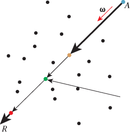
Three other phenomena arise for general participating media. The first of these is emission, shown by the red particle in the bottom left of the figure: Just as in the analysis of light’s interaction with surfaces, we can encounter media that glow (think of the liquid in glow sticks, or the heated soot in flame). The second is outscattering: Light hitting the medium may be scattered in various directions, causing things like the aforementioned shafts of light you see on a sunny day in a dusty room. This outscattering may not be uniform. Typically it’s assumed that the outscattering is constant as a function of course-deviation: If the light is traveling in direction ω, the probability of scattering to a new direction ω is assumed to be a function of ω·ω only. The third phenomenon is inscattering (shown at the green particle, just to the left of center in the diagram): Light scattered from other parts of the medium may arrive at some point and scatter so as to add the light we’re already observing. (Outscattered and inscattered light are therefore analogous to surface radiance and field radiance.)
These four effects can be combined to characterize how the radiance L(P, ω) at some point P in some direction ω is related to the radiance at P+ ω in direction ω; dividing the difference by ![]() and taking a limit as
and taking a limit as ![]()
![]() 0 gives an equation that L must satisfy, analogous to the rendering equation. Pharr and Humphreys [PH10] and Rushmeier [Rus08] give a great deal more detail on this subject.
0 gives an equation that L must satisfy, analogous to the rendering equation. Pharr and Humphreys [PH10] and Rushmeier [Rus08] give a great deal more detail on this subject.
The absorption constant σ has units of inverse meters. If light travels a distance of 1/σ through the absorbing medium, it’s attenuated by a factor of e. Perhaps more intuitive is that if the light travels 2.303/σ, it’s attenuated by a factor of 10. Even so, σ is not an intuitively easy-to-understand item. An artist is more likely to find 2.303/σ, the distance it takes to decrease by a factor of 10, to be a natural control for absorption.
The coefficient of extinction, κ, mentioned in Chapter 26 and sometimes used as the imaginary part of a complex index of refraction, is closely related to the absorption constant σ: It represents the exponential decay of the electromagnetic wave as it enters a homogeneous material. If we compute the absorption constant for the material at a particular wavelength ≠, the two are related by
Thus, the explicit dependence of absorption on wavelength is naturally incorporated by using κ. Of course, neither the idea of a complex index of refraction nor the coefficient of extinction is likely to be readily understood by a user; once again, the inverse of κ is likely to be more natural as a user control for material design. And for a material like smoke or fog, the absorption phenomenon is not really being governed by index-of-refraction effects, but by larger-scale phenomena, such as light entering and leaving the individual droplets of water in the fog.
27.13.2. Subsurface Scattering
In addition to mirrorlike reflections (and more diffuse reflections arising from multiple microfacets) and volumetric scattering, there’s a third kind of scattering that is very common: subsurface scattering.
In human skin, for instance, light meeting the skin at some point P may leave the skin at another point Q. To see this, sit in a dark room facing a mirror and place a small flashlight firmly against your cheek. You will see the skin around the flashlight glowing red because of subsurface conduction of the light. This cannot be modeled by a surface-based BSDF. Instead, we use a bidirectional subsurface scattering distribution function (BSSRDF), which has the form fss(P, Q, ωi, ωo), which represents the light leaving in direction vo from the point Q in response to light arriving from direction vi at point P (see Figure 27.19). It’s convenient to simplify things by assuming that the material is homogeneous and isotropic so that fss depends only on the distance from P to Q rather than on their absolute positions in the material; this substantially reduces the memory required to represent the scattering. But for many materials (like the palm of your hand), the geometric structure of the subsurface material is neither isotropic nor homogeneous. Things like veins, arteries, capillaries, muscle, cartilage, and fat all affect the scattering of light differently.
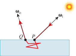
Figure 27.19: The arguments to the BSSRDF. The light enters the material at P from the source pointed to by ωi, travels along the red path, bouncing inside the material, and exits at Q in direction ωo.
How does the use of subsurface models influence the rendering equation? Recall that the basic model had the form
that is, the emitted radiance was basically the value of an integral over all incoming directions at P. But with subsurface scattering, light arriving at some other point Q might eventually be emitted at P, and the form becomes
Computing subsurface scattering adds another integral. In practice, for most materials the new integral (over all points Q of the material) can be replaced by one over a bounded area (like a disk) around P: Light entering at your fingertip is unlikely to exit at your nose in any substantial amount. If the material is homogeneous and isotropic, and the arriving radiance is nearly constant over the surface, the scattered radiance can be precomputed and stored in a lookup table, and the new computation is not much worse than that for the simpler rendering equation.
What are the practical effects of modeling subsurface scattering? First, it’s possible for light to diffuse across shadow boundaries so that a “hard shadow” on skin, for instance, ends up slightly softened. Second, it allows color bleeding within objects: A cup of tea with milk has its color affected, near the edge of the tea’s surface, by the color of the cup itself.
How does one model the subsurface scattering? In much the same way as we model surface scattering: either with acquired data, or by phenomenological or physical models. One can acquire data by modifying a gonioreflectometer to allow the sensor to be adjusted so that it measures light received from some location Q that’s not the center, P, of the sample stage—either by translating the entire sensor assembly in the plane of the sample stage, or by making a small, two-axis rotation of the sensor about its center. One could equally well translate or rotate the illumination source, of course, and/or rotate or translate the sample stage. Alternatively, one can illuminate the sample stage and then replace the usual sensor with a camera. This allows the measurement of light from many material points and directions at once. This approach is described by Jensen et al. [JMLH01] in some detail.
As for physical modeling of the subsurface scattering, it involves physics and mathematics well beyond the scope of this book. Jensen et al. describe some feasible approximations, and give a general overview and pointers to the physics literature.
27.14. Software Interface to Material Models
For our applications of material modeling to rendering, we’ll restrict our discussion to a particular class of models: those composed of a finite part and an impulse part, which we’ll now characterize.
The “impulse” part of scattering describes phenomena like transmission through boundaries between media, and mirror reflection: Radiance arriving from one single direction generates radiance leaving in a single other direction (or, in the case of simultaneous transmission and reflection, two other directions). These are the phenomena for which the measurement of the BSDF is impossible, as we described in Section 26.10.2. “Impulsive” scattering from ωi to ωo is described by a single factor by which incoming radiance is multiplied to produce outgoing radiance. We’ll assume that for a given direction ωi toward a light source, there are finitely many (usually two!) directions ωo for which (ωi, ωo) is an impulse-scattering pair. For each such pair, we’ll have a constant m, the magnitude of the impulse, which is the factor by which incoming radiance is multiplied to get outgoing radiance. Similarly, we’ll assume that if we know ωo, there are only finitely many directions ωi such that (ωi, ωo) is an impulse-scattering pair. To simplify things, for the remainder of this section we’ll say that there are exactly two impulse directions ![]() 1 and
1 and ![]() 2, with magnitudes m1 and m2.
2, with magnitudes m1 and m2.
When we want to ray-trace, it’s essential to recover these impulse directions and the associated material properties; we’ll need
ImpulseArray getImpulsesIn(surfel, ωo)
where surfel is a SurfaceElement data structure that stores the geometric normal at a point of some surface, the location of that point, the index of refraction of the material on the side pointed to by the normal and on the other side as well, and the shading normal (a vector used in shading computations, often interpolated from geometric normals at nearby points). The array of returned “impulses” contains a list of pairs (ω, ωo, m) where all the ωo values equal the input argument, and m is the magnitude of the impulse. It’s also useful to have the dual form
ImpulseArray getImpulsesOut(surfel, ωi)
which returns an array of (ωi, ω) pairs, together with their impulse magnitudes.
In fancier versions of ray tracing that can handle area lights and glossy surfaces, it’s also important to be able to evaluate the finite part of the BSDF for any two inputs, that is, we need
float getBSDFFinite(ωi,ωo)
It’s also useful to be able to “sample from the BSDF,” that is, to ask, given an output direction ωo, for an input direction ωi where the probability density of selecting ωi is proportional to fs(ωi, ωo). For a Lambertian surface, such a procedure would return a direction ωi in the upper hemisphere uniformly at random.
Sampling from the BSDF doesn’t make literal sense if the BSDF contains impulses, for in that case, certain BSDF values are infinite. Suppose, for instance, that we have a material and a direction-to-light ωi in which 40% of the light is mirror-reflected in a direction ![]() 1, while 60% is Lambertian-scattered. In this case, fs(ωi,
1, while 60% is Lambertian-scattered. In this case, fs(ωi, ![]() 1) = ∞, making sampling “proportional to” the BSDF impossible. But what we’d like, in this case, is for the sampling procedure to return
1) = ∞, making sampling “proportional to” the BSDF impossible. But what we’d like, in this case, is for the sampling procedure to return ![]() 1 40% of the time, and to return a vector ωi uniformly at random on the hemisphere the remaining 60% of the time. To further extend the example, if the magnitude of the impulse remained at 0.4, but the material absorbed 30% of the light hitting it and scattered the remaining 20% in a Lambertian fashion, we’d expect the procedure to return
1 40% of the time, and to return a vector ωi uniformly at random on the hemisphere the remaining 60% of the time. To further extend the example, if the magnitude of the impulse remained at 0.4, but the material absorbed 30% of the light hitting it and scattered the remaining 20% in a Lambertian fashion, we’d expect the procedure to return ![]() 1 40% of the time,
1 40% of the time, NONE 30% of the time, and a uniformly distributed random vector ωi the remaining 20% of the time. For this, we need a procedure like
Vector3 getSampleIn(ωo)
although such a procedure may, in the case of highly peaked BSDFs, prove to be very slow unless the material model has been designed in advance to make such sampling efficient.
Sometimes it suffices to get a sample where the probability density of a particular direction ωi isn’t exactly proportional to the BSDF fs(ωi, ωo), but whose probability distribution p is somewhat similarly shaped to the BSDF; in this case, we need to know not only the sample direction, but also a “factor” given by
although such an adjustment isn’t needed for the impulse terms, because they can be sampled from exactly. In this case, we need a procedure with a signature like
Vector3 getWeakSampleIn(ωo, float &factor)
in which the adjustment factor is set when the sampled vector is returned.
Corresponding procedures for sampling outgoing directions in proportion to the BSDF, or for sampling either incoming or outgoing directions in proportion to a cosine-weighted BSDF, are also useful. Indeed, the cosine-weighted versions are the ones we’ll primarily use in writing a path tracer and photon mapper in Chapter 32.
27.15. Discussion and Further Reading
Correctly modeling scattering is central to making renderings look realistic: For directly illuminated surfaces, our eyes essentially observe the BSDF, so making it right is important. Pharr and Humphreys [PH10] discuss the modeling of BSDFs, and a software interface to them, in extensive detail.
There’s a huge literature on scattering models, and it’s worth reading at least one or two of the early papers—perhaps the Torrance-Sparrow or Cook-Torrance or Blinn-Phong papers—to get an idea of all the complexities.
Lawrence [Law06] addresses the very practical question of how to make computational models for scattering that are (a) expressive enough to match measured data and (b) simple enough to admit relatively easy sampling strategies.
We began this chapter by discussing how objects transform light fields, and promptly shifted to talking about surfaces made of materials; this factorization is great for reducing the complexity of light transport (e.g., it lets us use the reflectance equation). But further factorization in the form of texture mapping, with parameters that can range from color to, say, the roughness parameter in some scattering model, allows further simplification. Appearance modeling is the craft of making compact representations for lots of materials. Given the messiness of scattering described in this chapter’s introduction, it should be no surprise that no general theory of appearance modeling has yet emerged, despite some substantial successes [GTR+06] [DRS08].
We briefly discussed volumetric scattering, with an implicit assumption that the distribution of particles in the scattering medium was uniform random. In cases where the distribution has some structure (e.g., the rings of Saturn), more sophisticated methods are called for. These were pioneered by Blinn [Bli82b], and advanced by Kajiya and von Herzen [KVH84], Miller [Mil88], and Kajiya and Kay [KK89], who introduced the notion of texels—three-dimensional arrays of parameters approximating the visual properties of microsurfaces like hair or fur—as a way to represent scattering of light from structured volumes of scatterers (see Figure 27.20). The complexities of that work demonstrate once again the point we made at the start of this chapter: Scattering tends to be messy and complex.

Figure 27.20: A teddy bear rendered by Kajiya and Kay’s texel-rendering algorithm. (Courtesy of Jim Kajiya. ©1989 ACM, Inc. Reprinted by permission.)
Is scattering too complex? If, in the course of rendering, we need to compute the light leaving some object but not going directly to the eye, it’s possible in many cases to use a simplified proxy for scattering: We can’t really tell whether light has been scattered from a furry teddy bear, or from a brown paper sack of about the same shape. There are exceptions, of course. Light scattered from a crystal chandelier produces highlights all around a room; replacing the crystals with diffusely scattering reflectors would not be the same at all. Even so, much of the effect of scattering—the complex appearance of the teddy bear, for instance—disappears after one bounce. It would be nice to avoid all the extra work in these cases.
In our discussion of the Torrance-Sparrow and Cook-Torrance models, scattering involves light inter-reflecting among multiple surfaces, resulting in shadowed and masked parts. This is exactly the same behavior we’ll see in studying global illumination algorithms, in which the geometry of a scene causes multiply reflected light to reach some places and not others. For real-time “solutions” (i.e., some games as of 2013), it turns out that we can approximate the effect of these complex global-illumination algorithms and replace them with the idea of ambient occlusion [Lan02], in which we make things darker when their surroundings are locally more convex, by setting an ambient term that’s proportional to how much of the far field you can see locally. This creates higher-frequency intensity gradients than you get with a 1/r2 falloff in light intensity, makes corners dark, and highlights concavities and convexities to give the viewer a clue about material smoothness at a relatively large scale, since shadows are an important proximity cue.
Finally, it’s worth standing back and looking at the microfacet models in a larger context. When we want to render a scene faithfully, we have to take into account how light from the luminaires scatters from each surface onto each other surface, and the resultant complex distribution of light energy reaching the eye or camera. The interconnectedness of all objects in the scene (or at least all mutually visible objects) leads to algorithmic complexity. Now look at microfacet models: They’re doing the same thing! Light arriving at the surface reaches only part of one microfacet because another shadows it, and light scattered from that microfacet hits yet another microfacet, etc. Because we’re assuming that the surfaces on which these microfacets reside are globally flat (at least relative to the scale of individual microfacets), we can assume that each microfacet interacts with only a few neighbors, thus reducing the complexity of the rendering problem. When we get to limiting cases like light arriving at a glancing angle, when many facets might shadow a single one, this simplifying assumption can break down.
27.16. Exercises
Exercise 27.1: In Gouraud shading, we have color values at the three vertices of a triangle, and we interpolate those values across the interior of the triangle. Since this is typically done on a raster screen, one approach is to work from top to bottom, linearly interpolating values along each edge, and then within a single row of pixels linearly interpolating between the two ends. In a typical triangle, there will be a top vertex, a bottom vertex, and a middle vertex. As we pass the middle vertex, we’ll need to start traversing a different edge. Alternatively, we could do interpolation from the top to the middle row, and from the bottom to the middle row.
(a) Show that if we compute the intersection of an edge with a row center exactly (rather than rounding to the nearest pixel center), the result is exactly the barycentric interpolation of the vertex values.
(b) Show that as we move from one row to the next, working down from the top vertex to the middle vertex, the starting value for each pixel row differs from the starting value for the previous row by the same amount.
(c) Use the idea of part (b) to develop a low-operation-count implementation of Gouraud shading in the 2D tested, using “pixels” that are each small, colored rectangles to visualize your results.
(d) Suppose we were to apply the same idea to shade a convex quadrilateral: We work from top to bottom, computing interpolated values along the two edge points in each row, and then linearly interpolate along the row. If we rotate the quadrilateral (keeping the assigned color values at each vertex), does the interpolated shading appear to rotate as well?
Exercise 27.2: It’s very common to photograph either the moon or a lighthouse being reflected in fairly calm (but not completely flat) water. The usual depiction shows the bright reflection appearing as a wedge that grows wider as it approaches the viewer, with the wedge point either near the lighthouse or (in the case of the moon) near the horizon. Find such a photograph, describe the notable features of the reflection (such as the shape of the wedge), and explain them in terms of the physical models you’ve seen in this chapter.
Exercise 27.3: A bookshelf holds three books, one with a white binding and two with black bindings. The shelf itself is made of polished wood. Looking down at the shelf, you can see the reflection of the spines of the books. Near the bottom of the spines, the division between the white and black reflections appears quite sharp. But if you look at the reflections of a region near the top of the spines, the division is quite blurry. Explain why. Is it a Fresnel effect, because of the difference in viewing angle? Why or why not? How could you test this idea? Hint: Actually set up the experiment!
Exercise 27.4: In the Phong model, as typically expressed, there’s a diffuse color, expressed as an RGB triple, and a diffuse reflectance.
(a) Make a conjecture about why these are not combined into a single RGB triple, since they are, after all, multiplied together in the model.
(b) The diffuse and specular colors in the Cook-Torrance model are specified by RGB triples (or more generally, by spectral distributions). Why do you suppose the specular exponent does not get expressed as an RGB triple?
(c) Suppose that the entire model was divided up by wavelength so that the specular exponent could vary from color to color. Suppose the red exponent was 3, while the blue and green exponents were 5, and that both the diffuse and specular colors were pure white. What would be the appearance of the specular highlight from a white point light?
Exercise 27.5: Plot FR, the Fresnel reflectance, as a function of θi, for an interface where r = n1/n2 is 1, 1.5, 2, and 3. To do so you’ll need to compute θt using Snell’s law.
Exercise 27.6: Compare the Schlick approximation of the reflectance with the Fresnel expression for the reflectance for aluminum and magnesium oxide at 500 nm. Magnesium oxide is nonmetallic, so the Schlick approximation should not necessarily be expected to work. Use 1.0 as the index of refraction of air, 1.44 for aluminum, and 1.74 for magnesium oxide.
Exercise 27.7: The Fresnel term used in graphics assumes that the arriving light is unpolarized; on the other hand, the different reflection constants for parallel and perpendicular polarization mean that the light leaving the surface is actually polarized. Yet we generally assume, when it reaches the next surface, that it’s unpolarized. Try to imagine a physical situation in which this inconsistency would manifest itself in a visible artifact.