
7.1 INTRODUCTION
This chapter discusses several ad hoc techniques used to implement parallel algorithms on parallel computers. Most of these techniques dealt with what is called embarrassingly parallel algorithms [2] or trivially parallel algorithms [29]. Parallel algorithms are expressed using loops. The simplest of these algorithms can be parallelized by assigning different iterations to different processors or even by assigning some of the operations in each iteration to different processors [29].
The techniques presented here do not deal efficiently with data dependencies. Unless the algorithm has no or very simple data dependence, it would be a challenge to correctly implement the algorithm in software using multithreading or in hardware using multiple processors. It will also be challenging to optimize interthread or interprocessor communications. In Chapters 9–11, we introduce formal techniques to deal with such algorithms. This chapter deals with what is termed “embarrassingly parallel” or “trivially parallel” algorithms. We should caution the reader, though, that some of these algorithms are far from trivial or embarrassingly simple. The full design space becomes apparent only by following the formal techniques discussed in Chapters 9–11. Take for example the algorithm for a one-dimensional (1-D) finite impulse response (FIR) digital filter given by the equation

where a(j) are the filter coefficients and I is the filter length. Such an equation is described by two nested loops as shown in Algorithm 7.1.
Algorithm 7.1
1-D FIR digital filter algorithm
Require: Input: filter coefficients a(n) and input samples x(n)
1: y(n) = 0
2: for i ≥ 0 do
3: y(i) = 0
4: for j = 0 : I − 1 do
5: y(i) = y(i) + a(j)x(i − j)
6: end for
7: RETURN y(i)
8: end for
The iterations in the nested loops are independent, and it is fairly easy to apply the techniques discussed here. However, these techniques only give one design option compared to the techniques in Chapters 9–11.
Take another example for a 1-D infinite impulse response (IIR) digital filter given by the equation
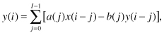
where a(j) and b(j) are the filter coefficients and I is the filter length. Note that b(0) = 0 in the above equation. Such an equation is described by two nested loops as shown in Algorithm 7.2.
Algorithm 7.2
1-D IIR digital filter algorithm
Require: Input: filter coefficients a(n) and b(n) and input samples x(n)
1: y(n) = 0
2: for i ≥ 0 do
3: y(i) = 0
4: for j = 0 : I − 1 do
5: y(i) = y(i) + a(j)x(i − j) − b(j)y(i − j)
6: end for
7: RETURN y(i)
8: end for
Although this algorithm has two simple nested FOR loops, the data dependencies within the loop body dictate that the evaluation of y(i) be serial. The techniques of this chapter will not be feasible here. However, the techniques of Chapters 9–11 will allow us to explore the possible parallelization techniques for this seemingly serial algorithm.