
Dinesh P. Mehta
Colorado School of Mines
Operations on an Array•Sorted Arrays•Array Doubling•Multiple Lists in a Single Array•Heterogeneous Arrays•Multidimensional Arrays•Sparse Matrices
Chains•Circular Lists•Doubly Linked Circular Lists•Generalized Lists
Stack Implementation•Queue Implementation
In this chapter, we review several basic structures that are usually taught in a first class on data structures. There are several text books that cover this material, some of which are listed here [1–4]. However, we believe that it is valuable to review this material for the following reasons:
1.In practice, these structures are used more often than all of the other data structures discussed in this handbook combined.
2.These structures are used as basic building blocks on which other more complicated structures are based.
Our goal is to provide a crisp and brief review of these structures. For a more detailed explanation, the reader is referred to the text books listed at the end of this chapter. In the following, we assume that the reader is familiar with arrays and pointers.
An array is conceptually defined as a collection of < index, value > pairs. The implementation of the array in modern programming languages such as C++ and Java uses indices starting at 0. Languages such as Pascal permitted one to define an array on an arbitrary range of integer indices. In most applications, the array is the most convenient method to store a collection of objects. In these cases, the index associated with a value is unimportant. For example, if an array city is being used to store a list of cities in no particular order, it doesn’t really matter whether city[0] is “Denver” or “Mumbai”. If, on the other hand, an array name is being used to store a list of student names in alphabetical order, then, although the absolute index values don’t matter, the ordering of names associated with the ordering of the index does matter: that is, name[i] must precede name[j] in alphabetical order, if i < j. Thus, one may distinguish between sorted arrays and unsorted arrays. Sometimes arrays are used so that the index does matter. For example, suppose we are trying to represent a histogram: we want to maintain a count of the number of students that got a certain score on an exam from a scale of 0 to 10. If score[5] = 7, this means that 7 students received a score of 5. In this situation, it is possible that the desired indices are not supported by the language. For example, C++ does not directly support using indices such as “blue”, “green”, and “red”. This may be rectified by using enumerated types to assign integer values to the indices. In cases when the objects in the array are large and unwieldy and have to be moved around from one array location to another, it may be advantageous to store pointers or references to objects in the array rather than the objects themselves.
Programming languages provide a mechanism to retrieve the value associated with a supplied index or to associate a value with an index. Programming languages like C++ do not explicitly maintain the size of the array. Rather, it is the programmer’s responsibility to be aware of the array size. Further, C++ does not provide automatic range-checking. Again, it is the programmer’s responsibility to ensure that the index being supplied is valid. Arrays are usually allocated contiguous storage in the memory. An array may be allocated statically (i.e., during compile-time) or dynamically (i.e., during program execution). For example, in C++, a static array is defined as:
int list[20];
while a dynamic one is defined as:
 int* list;
 .
 .
 list = new int[25];
An important difference between static and dynamic arrays is that the size of a static array cannot be changed during run time, while that of a dynamic array can (as we will see in Section 2.2.3).
1.Retrieval of an element: Given an array index, retrieve the corresponding value. This can be accomplished in O(1) time. This is an important advantage of the array relative to other structures. If the array is sorted, this enables one to compute the minimum, maximum, median (or in general, the ith smallest element) essentially for free in O(1) time.
2.Search: Given an element value, determine whether it is present in the array. If the array is unsorted, there is no good alternative to a sequential search that iterates through all of the elements in the array and stops when the desired element is found:
     int SequentialSearch(int* array, int n, int x)
     // search for x in array[n]
     {
         for (int i = 0; i < n; i++)
           if (array[i] == x) return i; // search succeeded
         return -1; // search failed
     }
In the worst case, this requires O(n) time. If, however, the array is sorted, binary search can be used.
     int BinarySearch(int* array, int n, int x)
     {
        int first = 0, mid, last = n-1;
        while (first < last) {
          mid = (first + last)/2;
          if (array[mid] == x) return mid; // search succeeded
          if (x < array[mid]) last = mid-1;
          else first = mid+1;
     }
      return -1; // search failed
    }
Binary search only requires O(log n) time.
3.Insertion and Deletion: These operations can be the array’s Achilles heel. First, consider a sorted array. It is usually assumed that the array that results from an insertion or deletion is to be sorted. The worst case scenario presents itself when an element that is smaller than all of the elements currently in the array is to be inserted. This element will be placed in the leftmost location. However, to make room for it, all of the existing elements in the array will have to be shifted one place to the right. This requires O(n) time. Similarly, a deletion from the leftmost element leaves a “vacant” location. Actually, this location can never be vacant because it refers to a word in memory which must contain some value. Thus, if the program accesses a “vacant” location, it doesn’t have any way to know that the location is vacant. It may be possible to establish some sort of code based on our knowledge of the values contained in the array. For example, if it is known that an array contains only positive integers, then one could use a zero to denote a vacant location. Because of these and other complications, it is best to eliminate vacant locations that are interspersed among occupied locations by shifting elements to the left so that all vacant locations are placed to the right. In this case, we know which locations are vacant by maintaining an integer variable which contains the number of locations starting at the left that are currently in use. As before, this shifting requires O(n) time. In an unsorted array, the efficiency of insertion and deletion depends on where elements are to be added or removed. If it is known for example that insertion and deletion will only be performed at the right end of the array, then these operations take O(1) time as we will see later when we discuss stacks.
We have already seen that there are several benefits to using sorted arrays, namely: searching is faster, computing order statistics (the ith smallest element) is O(1), etc. This is the first illustration of a key concept in data structures that will be seen several times in this handbook: the concept of preprocessing data to make subsequent queries efficient. The idea is that we are often willing to invest some time at the beginning in setting up a data structure so that subsequent operations on it become faster. Some sorting algorithms such as heap sort and merge sort require O(n log n) time in the worst case, whereas other simpler sorting algorithms such as insertion sort, bubble sort and selection sort require O(n2) time in the worst case. Others such as quick sort have a worst case time of O(n2), but require O(n log n) on the average. Radix sort requires Θ(n) time for certain kinds of data. We refer the reader to [5] for a detailed discussion.
However, as we have seen earlier, insertion into and deletion from a sorted array can take Θ(n) time, which is large. It is possible to merge two sorted arrays into a single sorted array in time linear in the sum of their sizes. However, the usual implementation needs additional Θ(n) space. See [6] for an O(1)-space merge algorithm.
To increase the length of a (dynamically allocated) one-dimensional array a that contains elements in positions a[0..n − 1], we first define an array of the new length (say m), then copy the n elements from a to the new array, and finally change the value of a so that it references the new array. It takes Θ(m) time to create an array of length m because all elements of the newly created array are initialized to a default value. It then takes an additional Θ(n) time to copy elements from the source array to the destination array. Thus, the total time required for this operation is Θ(m + n). This operation is used in practice to increase the array size when it becomes full. The new array is usually twice the length of the original; that is, m = 2n. The resulting complexity (Θ(n)) would normally be considered to be expensive. However, when this cost is amortized over the subsequent n insertions, it in fact only adds Θ(1) time per insertion. Since the cost of an insertion is Ω(1), this does not result in an asymptotic increase in insertion time. In general, increasing array size by a constant factor every time its size is to be increased does not adversely affect the asymptotic complexity. A similar approach can be used to reduce the array size. Here, the array size would be reduced by a constant factor every time.
2.2.4Multiple Lists in a Single Array
The array is wasteful of space when it is used to represent a list of objects that changes over time. In this scenario, we usually allocate a size greater than the number of objects that have to be stored, for example by using the array doubling idea discussed above. Consider a completely-filled array of length 8192 into which we are inserting an additional element. This insertion causes the array-doubling algorithm to create a new array of length 16,384 into which the 8192 elements are copied (and the new element inserted) before releasing the original array. This results in a space requirement during the operation which is almost three times the number of elements actually present. When several lists are to be stored, it is more efficient to store them all in a single array rather than allocating one array for each list.
Although this representation of multiple lists is more space-efficient, insertions can be more expensive because it may be necessary to move elements belonging to other lists in addition to elements in one’s own list. This representation is also harder to implement (Figure 2.1).

Figure 2.1Multiple lists in a single array.
The definition of an array in modern programming languages requires all of its elements to be of the same type. How do we then address the scenario where we wish to use the array to store elements of different types? In earlier languages like C, one could use the union facility to artificially coalesce the different types into one type. We could then define an array on this new type. The kind of object that an array element actually contains is determined by a tag. The following defines a structure that contains one of three types of data.
 struct Animal{
   int id;
   union {
     Cat c;
     Dog d;
     Fox f;
   }
 }
The programmer would have to establish a convention on how the id tag is to be used: for example, that id = 0 means that the animal represented by the struct is actually a cat, etc. The union allocates memory for the largest type among Cat, Dog, and Fox. This is wasteful of memory if there is a great disparity among the sizes of the objects. With the advent of object-oriented languages, it is now possible to define the base type Animal. Cat, Dog, and Fox may be implemented using inheritance as derived types of Animal. An array of pointers to Animal can now be defined. These pointers can be used to refer to any of Cat, Dog, and Fox.
2.2.6.1Row- or Column Major Representation
Earlier representations of multidimensional arrays mapped the location of each element of the multidimensional array into a location of a one- dimensional array. Consider a two-dimensional array with r rows and c columns. The number of elements in the array n = rc. The element in location [i][j], 0 ≤ i < r and 0 ≤ j < c, will be mapped onto an integer in the range [0, n − 1]. If this is done in row-major order — the elements of row 0 are listed in order from left to right followed by the elements of row 1, then row 2, etc. — the mapping function is ic + j. If elements are listed in column-major order, the mapping function is jr + i. Observe that we are required to perform a multiplication and an addition to compute the location of an element in an array.
2.2.6.2Array of Arrays Representation
In Java, a two-dimensional array is represented as a one-dimensional array in which each element is, itself, a one-dimensional array. The array
int [][] x = new int[4][5];
is actually a one-dimensional array whose length is 4. Each element of x is a one-dimensional array whose length is 5. Figure 2.2 shows an example. This representation can also be used in C++ by defining an array of pointers. Each pointer can then be used to point to a dynamically-created one-dimensional array. The element x[i][j] is found by first retrieving the pointer x[i]. This gives the address in memory of x[i][0]. Then x[i][j] refers to the element j in row i. Observe that this only requires the addition operator to locate an element in a one-dimensional array.
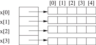
Figure 2.2The array of arrays representation.
2.2.6.3Irregular Arrays
A two-dimensional array is regular in that every row has the same number of elements. When two or more rows of an array have different number of elements, we call the array irregular. Irregular arrays may also be created and used using the array of arrays representation.
A matrix is sparse if a large number of its elements are 0. Rather than store such a matrix as a two-dimensional array with lots of zeroes, a common strategy is to save space by explicitly storing only the non-zero elements. This topic is of interest to the scientific computing community because of the large sizes of some of the sparse matrices it has to deal with. The specific approach used to store matrices depends on the nature of sparsity of the matrix. Some matrices, such as the tridiagonal matrix have a well-defined sparsity pattern. The tridiagonal matrix is one where all of the nonzero elements lie on one of three diagonals: the main diagonal and the diagonals above and below it. See Figure 2.3a.
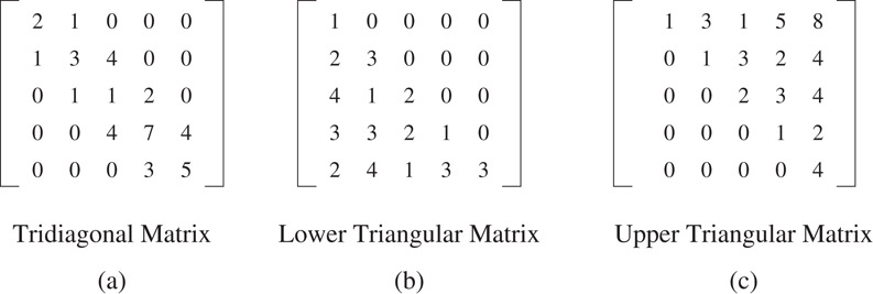
Figure 2.3Matrices with regular structures. (a) Tridiagonal Matrix, (b) Lower Triangular Matrix, (c) Upper Triangular Matrix.
There are several ways to represent this matrix as a one-dimensional array. We could order elements by rows giving [2,1,1,3,4,1,1,2,4,7,4,3,5] or by diagonals giving [1,1,4,3,2,3,1,7,5,1,4,2,4]. Figure 2.3 shows other special matrices: the upper and lower triangular matrices which can also be represented using a one-dimensional representation.
Other sparse matrices may have an irregular or unstructured pattern. Consider the matrix in Figure 2.4a. We show two representations. Figure 2.4b shows a one-dimensional array of triples, where each triple represents a nonzero element and consists of the row, column, and value. Figure 2.4c shows an irregular array representation. Each row is represented by a one-dimensional array of pairs, where each pair contains the column number and the corresponding nonzero value.
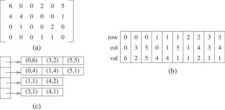
Figure 2.4Unstructured matrices.
The linked list is an alternative to the array when a collection of objects is to be stored. The linked list is implemented using pointers. Thus, an element (or node) of a linked list contains the actual data to be stored and a pointer to the next node. Recall that a pointer is simply the address in memory of the next node. Thus, a key difference from arrays is that a linked list does not have to be stored contiguously in memory.
The code fragment below defines a linked list data structure, which is also illustrated in Figure 2.5:
 class ListNode {
 friend class List;
 private:
   int data;
   ListNode *link;
 }
 class List {
 public:
  // List manipulation operations go here
  ...
 private:
  ListNode *first;
 }
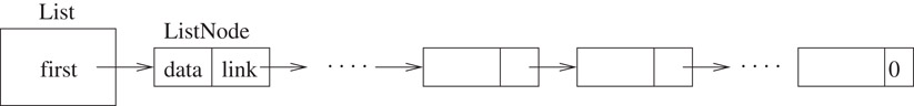
Figure 2.5The structure of a linked list.
A chain is a linked list where each node contains a pointer to the next node in the list. The last node in the list contains a null (or zero) pointer. A circular list is identical to a chain except that the last node contains a pointer to the first node. A doubly linked circular list differs from the chain and the circular list in that each node contains two pointers. One points to the next node (as before), while the other points to the previous node.
The following code searches for a key k in a chain and returns true if the key is found and false, otherwise.
 bool List::Search(int k) {
  for (ListNode *current = first; current; current = current->next)
    if (current->data == k) then return true;
  return false;
 }
In the worst case, Search takes Θ(n) time. In order to insert a node newnode in a chain immediately after node current, we simply set newnode’s pointer to the node following current (if any) and current’s pointer to newnode as shown in the Figure 2.6.
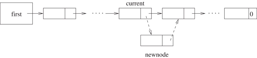
Figure 2.6Insertion into a chain. The dashed links show the pointers after newnode has been inserted.
To delete a node current, it is necessary to have a pointer to the node preceding current. This node’s pointer is then set to current->next and node current is freed. Both insertion and deletion can be accomplished in O(1) time provided that the required pointers are initially available. Whether this is true or not depends on the context in which these operations are called. For example, if you are required to delete the node with key 50, if it exists, from a linked list, you would first have to search for 50. Your search algorithm would maintain a trailing pointer so that when 50 is found, a pointer to the previous node is available. Even though, deletion takes Θ(1) time, deletion in this context would require Θ(n) time in the worst case because of the search. In some cases, the context depends on how the list is organized. For example, if the list is to be sorted, then node insertions should be made so as to maintain the sorted property (which could take Θ(n) time). On the other hand, if the list is unsorted, then a node insertion can take place anywhere in the list. In particular, the node could be inserted at the front of the list in Θ(1) time. Interestingly, the author has often seen student code in which the insertion algorithm traverses the entire linked list and inserts the new element at the end of the list!
As with arrays, chains can be sorted or unsorted. Unfortunately, however, many of the benefits of a sorted array do not extend to sorted linked lists because arbitrary elements of a linked list cannot be accessed quickly. In particular, it is not possible to carry out binary search in O(log n) time. Nor is it possible to locate the ith smallest element in O(1) time. On the other hand, merging two sorted lists into one sorted list is more convenient than merging two sorted arrays into one sorted array because the traditional implementation requires space to be allocated for the target array. A code fragment illustrating the merging of two sorted lists is shown below. This is a key operation in mergesort:
 void Merge(List listOne, List listTwo, List& merged) {
  ListNode* one = listOne.first;
  ListNode* two = listTwo.first;
  ListNode* last = 0;

  if (one == 0) {merged.first = two; return;}
  if (two == 0) {merged.first = one; return;}

  if (one->data < two->data) last = merged.first = one;
  else last = merged.first = two;
  while (one && two)
     if (one->data < two->data) {
      last->next = one; last= one; one = one->next;
     }
     else {
      last->next = two; last = two; two = two->next;
     }
  if (one) last->next = one;
  else last->next = two;
 }
The merge operation is not defined when lists are unsorted. However, one may need to combine two lists into one. This is the concatenation operation. With chains, the best approach is to attach the second list to the end of the first one. In our implementation of the linked list, this would require one to traverse the first list until the last node is encountered and then set its next pointer to point to the first element of the second list. This requires time proportional to the size of the first linked list. This can be improved by maintaining a pointer to the last node in the linked list.
It is possible to traverse a singly linked list in both directions (i.e., left to right and a restricted right-to-left traversal) by reversing links during the left-to-right traversal. Figure 2.7 shows a possible configuration for a list under this scheme.
As with the heterogeneous arrays described earlier, heterogeneous lists can be implemented in object-oriented languages by using inheritance.
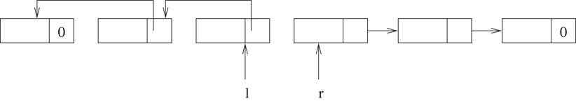
Figure 2.7Illustration of a chain traversed in both directions.
In the previous section, we saw that to concatenate two unsorted chains efficiently, one needs to maintain a rear pointer in addition to the first pointer. With circular lists, it is possible to accomplish this with a single pointer as follows: consider the circular list in Figure 2.8. The second node in the list can be accessed through the first in O(1) time. Now, consider the list that begins at this second node and ends at the first node. This may be viewed as a chain with access pointers to the first and last nodes. Concatenation can now be achieved in O(1) time by linking the last node of one chain to the first node of the second chain and vice versa.
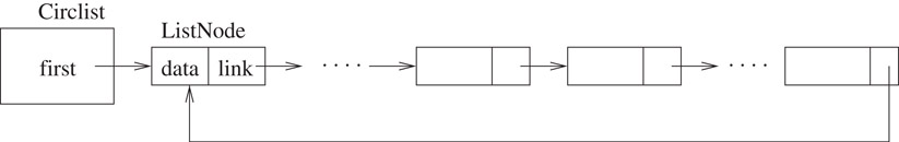
Figure 2.8A circular list.
2.3.3Doubly Linked Circular Lists
A node in a doubly linked list differs from that in a chain or a singly linked list in that it has two pointers. One points to the next node as before, while the other points to the previous node. This makes it possible to traverse the list in both directions. We observe that this is possible in a chain as we saw in Figure 2.7. The difference is that with a doubly linked list, one can initiate the traversal from any arbitrary node in the list. Consider the following problem: we are provided a pointer x to a node in a list and are required to delete it as shown in Figure 2.9. To accomplish this, one needs to have a pointer to the previous node. In a chain or a circular list, an expensive list traversal is required to gain access to this previous node. However, this can be done in O(1) time in a doubly linked circular list. The code fragment that accomplishes this is as below:
 void DblList::Delete(DblListNode* x)
 {
  x->prev->next = x->next;
  x->next->prev = x->prev;
  delete x;
 }
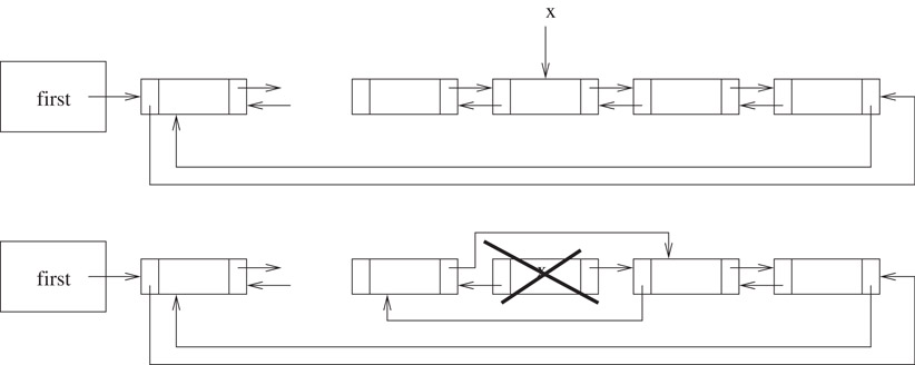
Figure 2.9Deletion from a doubly linked list.
An application of doubly linked lists is to store a list of siblings in a Fibonacci heap (Chapter 7).
A generalized list A is a finite sequence of n ≥ 0 elements, e0, e1,…, en − 1, where ei is either an atom or a generalized list. The elements ei that are not atoms are said to be sublists of A. Consider the generalized list A = ((a, b, c),((d, e), f), g). This list contains three elements: the sublist (a, b, c), the sublist ((d, e), f) and the atom g. The generalized list may be implemented by employing a GenListNode type as follows:
 private:
  GenListNode* next;
  bool tag;
  union {
    char data;
    GenListNode* down;
  };
If tag is true, the element represented by the node is a sublist and down points to the first node in the sublist. If tag is false, the element is an atom whose value is contained in data. In both cases, next simply points to the next element in the list. Figure 2.10 illustrates the representation.
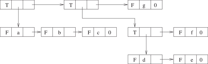
Figure 2.10Generalized list for ((a,b,c),((d,e),f),g).
The stack and the queue are data types that support insertion and deletion operations with well-defined semantics. Stack deletion deletes the element in the stack that was inserted the last, while a queue deletion deletes the element in the queue that was inserted the earliest. For this reason, the stack is often referred to as a LIFO (Last In First Out) data type and the queue as an FIFO (First In First out) data type. A deque (double ended queue) combines the stack and the queue by supporting both types of deletions.
Stacks and queues find a lot of applications in Computer Science. For example, a system stack is used to manage function calls in a program. When a function f is called, the system creates an activation record and places it on top of the system stack. If function f calls function g, the local variables of f are added to its activation record and an activation record is created for g. When g terminates, its activation record is removed and f continues executing with the local variables that were stored in its activation record. A queue is used to schedule jobs at a resource when a first-in first-out policy is to be implemented. Examples could include a queue of print-jobs that are waiting to be printed or a queue of packets waiting to be transmitted over a wire. Stacks and queues are also used routinely to implement higher-level algorithms. For example, a queue is used to implement a breadth-first traversal of a graph. A stack may be used by a compiler to process an expression such as (a + b) × (c + d).
Stacks and queues can be implemented using either arrays or linked lists. Although the burden of a correct stack or queue implementation appears to rest on deletion rather than insertion, it is convenient in actual implementations of these data types to place restrictions on the insertion operation as well. For example, in an array implementation of a stack, elements are inserted in a left-to-right order. A stack deletion simply deletes the rightmost element.
A simple array implementation of a stack class is shown below:
 class Stack {
 public:
     Stack(int maxSize = 100); // 100 is default size
  void Insert(int);
  int* Delete(int&);
 private:
  int *stack;
  int size;
  int top; // highest position in array that contains an element
 };
The stack operations are implemented as follows:
 Stack::Stack(int maxSize): size(maxSize)
 {
  stack = new int[size];
  top = -1;
 }

 void Stack::Insert(int x)
 {
  if (top == size-1) cerr << "Stack Full" << endl;
  else stack[++top] = x;
 }

 int* Stack::Delete(int& x)
 {
  if (top == -1) return 0; // stack empty
  else {
    x = stack[top--];
    return &x;
  }
 }
The operation of the following code fragment is illustrated in Figure 2.11.
 Stack s;
 int x;
 s.Insert(10);
 s.Insert(20);
 s.Insert(30);
 s.Delete(x);
 s.Insert(40);
 s.Delete(x);
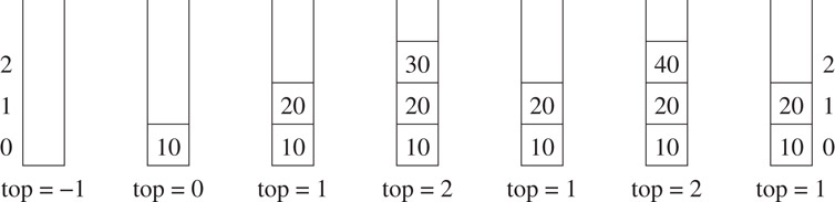
Figure 2.11Stack operations.
It is easy to see that both stack operations take O(1) time. The stack data type can also be implemented using linked lists by requiring all insertions and deletions to be made at the front of the linked list.
An array implementation of a queue is a bit trickier than that of a stack. Insertions can be made in a left-to-right fashion as with a stack. However, deletions must now be made from the left. Consider a simple example of an array of size 5 into which the integers 10, 20, 30, 40, and 50 are inserted as shown in Figure 2.12a. Suppose three elements are subsequently deleted (Figure 2.12b).
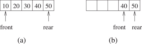
Figure 2.12Pitfalls of a simple array implementation of a queue.
What if we are now required to insert the integer 60. On one hand, it appears that we are out of room as there is no more place to the right of 50. On the other hand, there are three locations available to the left of 40. This suggests that we use a circular array implementation of a queue, which is described below.
 class Queue {
 public:
     Queue(int maxSize = 100); // 100 is default size
  void Insert(int);
  int* Delete(int&);
 private:
  int *queue;
  int size;
  int front, rear;
 };
The queue operations are implemented below:
 Queue::Queue(int maxSize): size(maxSize)
 {
  queue= new int[size];
  front = rear = 0;
 }

 void Queue::Insert(int x)
 {
  int k = (rear + 1)
  if (front == k) cerr << "Queue Full!" <, endl;
  else queue[rear = k] = x;
 }

 int* Queue::Delete(int& x)
 {
  if (front == rear) return 0; // queue is empty
  x = queue[++front
  return &x;
 }
Figure 2.13 illustrates the operation of this code on an example. The first figure shows an empty queue with first = rear = 0. The second figure shows the queue after the integer 10 is inserted. The third figure shows the queue when 20, 30, 40, 50, and 60 have been inserted. The fourth figure shows the queue after 70 is inserted. Notice that, although one slot remains empty, the queue is now full because Queue::Insert will not permit another element to be inserted. If it did permit an insertion at this stage, rear and front would be the same. This is the condition that Queue:Delete checks to determine whether the queue is empty! This would make it impossible to distinguish between the queue being full and being empty. The fifth figure shows the queue after two integers (10 and 20) are deleted. The last figure shows a full queue after the insertion of integers 80 and 90.
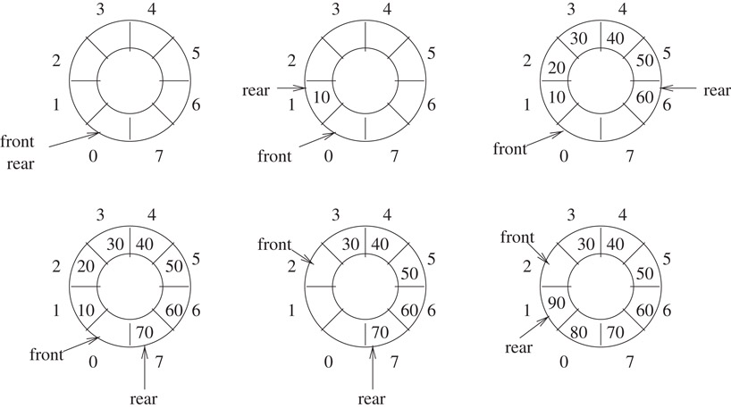
Figure 2.13Implementation of a queue in a circular array.
It is easy to see that both queue operations take O(1) time. The queue data type can also be implemented using linked lists by requiring all insertions and deletions to be made at the front of the linked list.
The author would like to thank Kun Gao, Dean Simmons and Mr. U. B. Rao for proofreading this chapter. This work was supported, in part, by the National Science Foundation under grant CCR-9988338.
1.D. Knuth, The Art of Computer Programming, Vol. 1, Fundamental Algorithms, Third edition. Addison-Wesley, NY, 1997.
2.S. Sahni, Data Structures, Algorithms, and Applications in C++, McGraw-Hill, NY, 1998.
3.S. Sahni, Data Structures, Algorithms, and Applications in Java, McGraw-Hill, NY, 2000.
4.E. Horowitz, S. Sahni, and D. Mehta, Fundamentals of Data Structures in C++, W. H. Freeman, NY, 1995.
5.D. Knuth, The Art of Computer Programming, Vol. 3, Sorting and Searching, Second edition. Addison-Wesley, NY, 1997.
6.B. Huang and M. Langston, Practical in-place merging, Communications of the ACM, 31:3, 1988, pp. 348–352.
*This chapter has been reprinted from first edition of this Handbook, without any content updates.