
Dinesh P. Mehta
Colorado School of Mines
List Representation•Left Child-Right Sibling Representation•Binary Tree Representation
3.3Binary Trees and Properties
Properties•Binary Tree Representation
Inorder Traversal•Preorder Traversal•Postorder Traversal•Level Order Traversal
Threads•Inorder Traversal of a Threaded Binary Tree
Definition•Search•Insert•Delete•Miscellaneous
Priority Queues•Definition of a Max-Heap•Insertion•Deletion
The tree is a natural representation for hierarchical information. Thus, trees are used to represent genealogical information (e.g., family trees and evolutionary trees), organizational charts in large companies, the directory structure of a file system on a computer, parse trees in compilers and the structure of a knock-out sports tournament. The Dewey decimal notation, which is used to classify books in a library, is also a tree structure. In addition to these and other applications, the tree is used to design fast algorithms in computer science because of its efficiency relative to the simpler data structures discussed in Chapter 2. Operations that take linear time on these structures often take logarithmic time on an appropriately organized tree structure. For example, the average time complexity for a search on a key is linear on a linked list and logarithmic on a binary search tree. Many of the data structures discussed in succeeding chapters of this handbook are tree structures.
Several kinds of trees have been defined in the literature:
1.Free or unrooted tree: this is defined as a graph (a set of vertices and a set of edges that join pairs of vertices) such that there exists a unique path between any two vertices in the graph. The minimum spanning tree of a graph is a well-known example of a free tree. Graphs are discussed in Chapter 4.
2.Rooted tree: a finite set of one or more nodes such that
a.There is a special node called the root.
b.The remaining nodes are partitioned into n ≥ 0 disjoint sets T1,…, Tn, where each of these sets is a tree. T1,…, Tn are called the subtrees of the root.
If the order in which the subtrees are arranged is not important, then the tree is a rooted, unordered (or oriented) tree. If the order of the subtrees is important, the tree is rooted and ordered. Figure 3.1 depicts the relationship between the three types of trees. We will henceforth refer to the rooted, ordered tree simply as “tree.”
3.k-ary tree: a finite set of nodes that is either empty or consists of a root and the elements of k disjoint k-ary trees called the 1st, 2nd, …, kth subtrees of the root. The binary tree is a k-ary tree with k = 2. Here, the first and second subtrees are respectively called the left and right subtrees of the root. Note that binary trees are not trees. One difference is that a binary tree can be empty, whereas a tree cannot. Second, the two trees shown in Figure 3.2 are different binary trees but would be different drawings of the same tree.
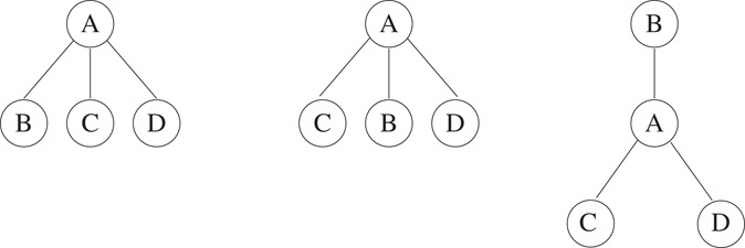
Figure 3.1The three trees shown are distinct if they are viewed as rooted, ordered trees. The first two are identical if viewed as oriented trees. All three are identical if viewed as free trees.
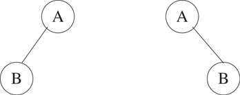
Figure 3.2Different binary trees.
Figure 3.3 shows a tree with 11 nodes. The number of subtrees of a node is its degree. Nodes with degree 0 are called leaf nodes. Thus, node A has degree 3, nodes B, D, and I have degree 2, node E has degree 1, and nodes C, F, G, H, J, and K have degree 0 (and are leaves of the tree). The degree of a tree is the maximum of the degree of the nodes in the tree. The roots of the subtrees of a node X are its children. X is the parent of its children. Children of the same parent are siblings. In the example, B, C, and D are each other’s siblings and are all children of A. The ancestors of a node are all the nodes excluding itself along the path from the root to that node. The level of a node is defined by letting the root be at level zero. If a node is at level l, then its children are at level l + 1. The height of a tree is the maximum level of any node in the tree. The tree in the example has height 4. These terms are defined in the same way for binary trees. See [1–6] for more information on trees.
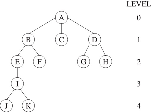
Figure 3.3An example tree.
The tree of Figure 3.3 can be written as the generalized list (A (B (E (I (J, K)), F), C, D(G, H))). The information in the root node comes first followed by a list of subtrees of the root. This enables us to represent a tree in memory using generalized lists as discussed in Chapter 2.
3.2.2Left Child-Right Sibling Representation
Figure 3.4a shows the node structure used in this representation. Each node has a pointer to its leftmost child (if any) and to the sibling on its immediate right (if any). The tree in Figure 3.3 is represented by the tree in Figure 3.4b.
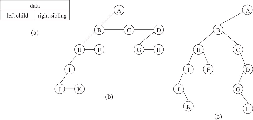
Figure 3.4Tree representations.
3.2.3Binary Tree Representation
Observe that the left child-right sibling representation of a tree (Figure 3.4b) may be viewed as a binary tree by rotating it clockwise by 45 degrees. This gives the binary tree representation shown in Figure 3.4c. This representation can be extended to represent a forest, which is defined as an ordered set of trees. Here, the roots of the trees are viewed as siblings. Thus, a root’s right pointer points to the next tree root in the set. We have
Lemma 3.1
There is a one-to-one correspondence between the set of forests and the set of binary trees.
3.3Binary Trees and Properties
Binary trees were defined in Section 3.1. For convenience, a binary tree is sometimes extended by adding external nodes. External nodes are imaginary nodes that are added wherever an empty subtree was present in the original tree. The original tree nodes are known as internal nodes. Figure 3.5a shows a binary tree and (b) the corresponding extended tree. Observe that in an extended binary tree, all internal nodes have degree 2 while all external nodes have degree 0. (Some authors use the term full binary tree to denote a binary tree whose nodes have 0 or two children.) The external path length of a tree is the sum of the lengths of all root-to-external node paths in the tree. In the example, this is 2 + 2 + 3 + 3 + 2 = 12. The internal path length is similarly defined by adding lengths of all root-to-internal node paths. In the example, this quantity is 0 + 1 + 1 + 2 = 4.
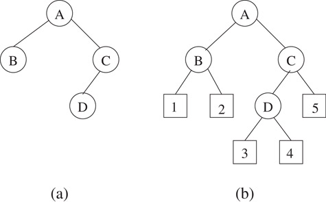
Figure 3.5(b) shows the extended binary tree corresponding to the binary tree of (a). External nodes are depicted by squares.
Lemma 3.2
A binary tree with n internal nodes has n + 1 external nodes.
Proof. Each internal node in the extended tree has branches leading to two children. Thus, the total number of branches is 2n. Only n − 1 internal nodes have a single incoming branch from a parent (the root does not have a parent). Thus, each of the remaining n + 1 branches points to an external node.■
Lemma 3.3
For any non-empty binary tree with n0 leaf nodes and n2 nodes of degree 2, n0 = n2 + 1.
Proof. Let n1 be the number of nodes of degree 1 and n = n0 + n1 + n2 (Equation 1) be the total number of nodes. The number of branches in a binary tree is n − 1 since each non-root node has a branch leading into it. But, all branches stem from nodes of degree 1 and 2. Thus, the number of branches is n1 + 2n2. Equating the two expressions for number of branches, we get n = n1 + 2n2 + 1 (Equation 2). From Equations 1 and 2, we get n0 = n2 + 1.■
Lemma 3.4
The external path length of any binary tree with n internal nodes is 2n greater than its internal path length.
Proof. The proof is by induction. The lemma clearly holds for n = 0 when the internal and external path lengths are both zero. Consider an extended binary tree T with n internal nodes. Let ET and IT denote the external and internal path lengths of T. Consider the extended binary tree S that is obtained by deleting an internal node whose children are both external nodes (i.e., a leaf) and replacing it with an external node. Let the deleted internal node be at level l. Thus, the internal path length decreases by l while the external path length decreases by 2(l + 1)−l = l + 2. From the induction hypothesis, ES = IS + 2(n−1). But, ET = ES + l + 2 and IT = IS + l. Thus, ET − IT = 2n.■
Lemma 3.5
The maximum number of nodes on level i of a binary tree is 2i, i ≥ 0.
Proof. This is easily proved by induction on i.■
Lemma 3.6
The maximum number of nodes in a binary tree of height k is 2k + 1− 1.
Proof. Each level i, 0 ≤ i ≤ k, has 2i nodes. Summing over all i results in .■
Lemma 3.7
The height of a binary tree with n internal nodes is at least ⌈ log2(n + 1)⌉ and at most n − 1.
Proof. The worst case is a skewed tree (Figure 3.6a) and the best case is a tree with 2i nodes at every level i except possibly the bottom level (Figure 3.6b). If the height is h, then n + 1 ≤ 2h, where n + 1 is the number of external nodes.■
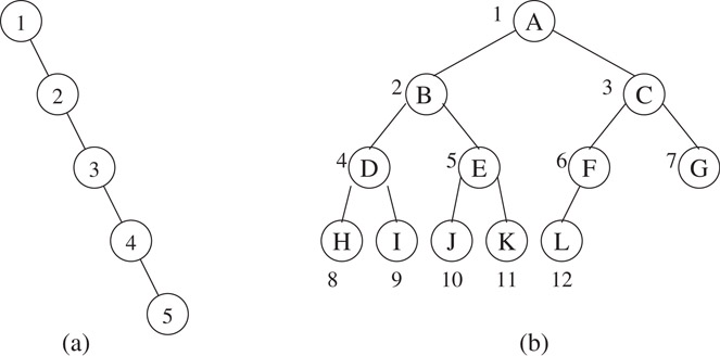
Figure 3.6(a) Skewed and (b) complete binary trees.
Lemma 3.8
The number of distinct binary trees with n nodes is .
Proof. For a detailed proof, we refer the reader to [7]. However, we note that are known as the Catalan numbers, which occur frequently in combinatorial problems. The Catalan number Cn also describes the number of trees with n + 1 nodes and the number of binary trees with 2n + 1 nodes all of which have 0 or 2 children.■
3.3.2Binary Tree Representation
Binary trees are usually represented using nodes and pointers. A TreeNode class may be defined as:
 class TreeNode {
   TreeNode* LeftChild;
   TreeNode* RightChild;
   KeyType data;
 };
In some cases, a node might also contain a parent pointer which facilitates a “bottom-up” traversal of the tree. The tree is accessed by a pointer root of type TreeNode* to its root. When the binary tree is complete (i.e., there are 2i nodes at every level i, except possibly the last level which has nodes filled in from left to right), it is convenient to use an array representation. The complete binary tree in Figure 3.6b can be represented by the array
   1 2 3 4 5 6 7 8 9 10 11 12
 [ A B C D E F G H I J  K  L ]
Observe that the children (if any) of a node located at position i of the array can be found at positions 2i and 2i + 1 and its parent at ⌊i/2⌋.
Several operations on trees require one to traverse the entire tree: that is, given a pointer to the root of a tree, process every node in the tree systematically. Printing a tree is an example of an operation that requires a tree traversal. Starting at a node, we can do one of three things: visit the node (V), traverse the left subtree recursively (L), and traverse the right subtree recursively (R). If we adopt the convention that the left subtree will be visited before the right subtree, we have three types of traversals LV R, V LR, and LRV which are called inorder, preorder, and postorder, respectively, because of the position of V with respect to L and R. In the following, we will use the expression tree in Figure 3.7 to illustrate the three traversals, which result in infix, prefix, and postfix forms of the expression. A fourth traversal, the level order traversal, is also studied.
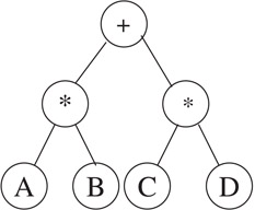
Figure 3.7An expression tree.
The following is a recursive algorithm for an inorder traversal that prints the contents of each node when it is visited. The recursive function is invoked by the call inorder(root). When run on the example expression tree, it returns A*B+C*D.
 inorder(TreeNode* currentNode)
 {
   if (currentNode) {
    inorder(currentNode->LeftChild);
    cout << currentNode->data;
    inorder(currentNode->RightChild);
   }
 }
The following is a recursive algorithm for a preorder traversal that prints the contents of each node when it is visited. The recursive function is invoked by the call preorder(root). When run on the example expression tree, it returns +*AB*CD.
 preorder(TreeNode* currentNode)
 {
   if (currentNode) {
     cout << currentNode->data;
     preorder(currentNode->LeftChild);
     preorder(currentNode->RightChild);
   }
 }
The following is a recursive algorithm for a postorder traversal that prints the contents of each node when it is visited. The recursive function is invoked by the call postorder(root). When run on the example expression tree, it prints AB*CD*+.
 postorder(TreeNode* currentNode)
 {
   if (currentNode) }
     postorder(currentNode->LeftChild);
     postorder(currentNode->RightChild);
     cout << currentNode->data;
   }
 }
The complexity of each of the three algorithms is linear in the number of tree nodes. Non-recursive versions of these algorithms may be found in Reference 6. Both versions require (implicitly or explicitly) a stack.
The level order traversal uses a queue. This traversal visits the nodes in the order suggested in Figure 3.6b. It starts at the root and then visits all nodes in increasing order of their level. Within a level, the nodes are visited in left-to-right order.
 LevelOrder(TreeNode* root)
 {
   Queue q<TreeNode*>;
   TreeNode* currentNode = root;
   while (currentNode) {
     cout << currentNode->data;
     if (currentNode->LeftChild) q.Add(currentNode->LeftChild);
     if (currentNode->RightChild) q.Add(currentNode->RightChild);
     currentNode = q.Delete(); //q.Delete returns a node pointer
   }
 }
Lemma 3.2 implies that a binary tree with n nodes has n + 1 null links. These null links can be replaced by pointers to nodes called threads. Threads are constructed using the following rules:
1.A null right child pointer in a node is replaced by a pointer to the inorder successor of p (i.e., the node that would be visited after p when traversing the tree inorder).
2.A null left child pointer in a node is replaced by a pointer to the inorder predecessor of p.
Figure 3.8 shows the binary tree of Figure 3.7 with threads drawn as broken lines. In order to distinguish between threads and normal pointers, two boolean fields LeftThread and RightThread are added to the node structure. If p->LeftThread is 1, then p->LeftChild contains a thread; otherwise it contains a pointer to the left child. Additionally, we assume that the tree contains a head node such that the original tree is the left subtree of the head node. The LeftChild pointer of node A and the RightChild pointer of node D point to the head node.
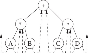
Figure 3.8A threaded binary tree.
3.5.2Inorder Traversal of a Threaded Binary Tree
Threads make it possible to perform an inorder traversal without using a stack. For any node p, if p’s right thread is 1, then its inorder successor is p->RightChild. Otherwise the inorder successor is obtained by following a path of left-child links from the right child of p until a node with left thread 1 is reached. Function Next below returns the inorder successor of currentNode (assuming that currentNode is not 0). It can be called repeatedly to traverse the entire tree in inorder in O(n) time. The code below assumes that the last node in the inorder traversal has a threaded right pointer to a dummy head node.
 TreeNode* Next(TreeNode* currentNode)
 {
   TreeNode* temp = currentNode->RightChild;
   if (currentNode->RightThread == 0)
     while (temp->LeftThread == 0)
       temp = temp->LeftChild;
   currentNode = temp;
   if (currentNode == headNode)
     return 0;
   else
     return currentNode;
 }
Threads simplify the algorithms for preorder and postorder traversal. It is also possible to insert a node into a threaded tree in O(1) time [6].
A binary search tree (BST) is a binary tree that has a key associated with each of its nodes. The keys in the left subtree of a node are smaller than or equal to the key in the node and the keys in the right subtree of a node are greater than or equal to the key in the node. To simplify the discussion, we will assume that the keys in the binary search tree are distinct. Figure 3.9 shows some binary trees to illustrate the definition.
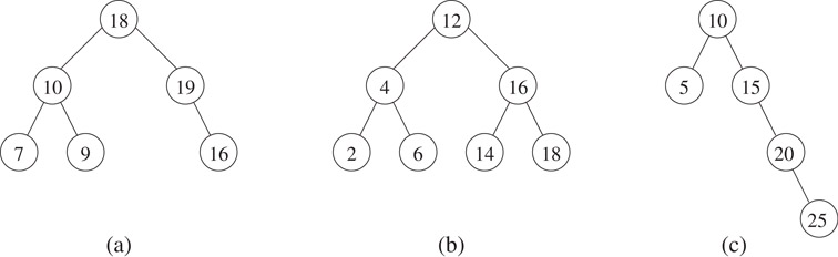
Figure 3.9Binary trees with distinct keys: (a) is not a BST. (b) and (c) are BSTs.
We describe a recursive algorithm to search for a key k in a tree T: first, if T is empty, the search fails. Second, if k is equal to the key in T’s root, the search is successful. Otherwise, we search T’s left or right subtree recursively for k depending on whether it is less or greater than the key in the root.
 bool Search(TreeNode* b, KeyType k)
 {
   if (b == 0) return 0;
   if (k == b->data) return 1;
   if (k < b->data) return Search(b->LeftChild,k);
   if (k > b->data) return Search(b->RightChild,k);
 }
To insert a key k, we first carry out a search for k. If the search fails, we insert a new node with k at the null branch where the search terminated. Thus, inserting the key 17 into the binary search tree in Figure 3.9b creates a new node which is the left child of 18. The resulting tree is shown in Figure 3.10a.
 typedef TreeNode* TreeNodePtr;

 Node* Insert(TreeNodePtr& b, KeyType k)
 {
   if (b == 0) {b = new TreeNode; b->data= k; return b;}
   if (k == b->data) return 0; // don’t permit duplicates
   if (k < b->data) Insert(b->LeftChild, k);
   if (k > b->data) Insert(b->RightChild, k);
 }
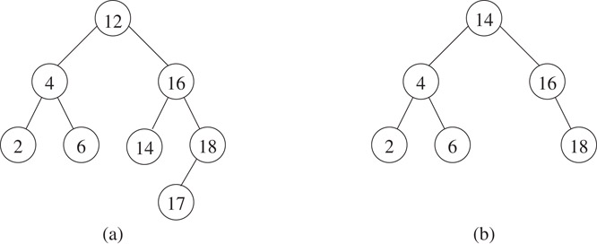
Figure 3.10Tree of Figure 3.9b with (a) 18 inserted and (b) 12 deleted.
The procedure for deleting a node x from a binary search tree depends on its degree. If x is a leaf, we simply set the appropriate child pointer of x’s parent to 0 and delete x. If x has one child, we set the appropriate pointer of x’s parent to point directly to x’s child and then delete x. In Figure 3.9c, node 20 is deleted by setting the right child of 15 to 25. If x has two children, we replace its key with the key in its inorder successor y and then delete node y. The inorder successor contains the smallest key greater than x’s key. This key is chosen because it can be placed in node x without violating the binary search tree property. Since y is obtained by first following a RightChild pointer and then following LeftChild pointers until a node with a null LeftChild pointer is encountered, it follows that y has degree 0 or 1. Thus, it is easy to delete y using the procedure described above. Consider the deletion of 12 from Figure 3.9b. This is achieved by replacing 12 with 14 in the root and then deleting the leaf node containing 14. The resulting tree is shown in Figure 3.10b.
Although Search, Insert, and Delete are the three main operations on a binary search tree, there are others that can be defined which we briefly describe below.
•Minimum and Maximum that respectively find the minimum and maximum elements in the binary search tree. The minimum element is found by starting at the root and following LeftChild pointers until a node with a 0 LeftChild pointer is encountered. That node contains the minimum element in the tree.
•Another operation is to find the kth smallest element in the binary search tree. For this, each node must contain a field with the number of nodes in its left subtree. Suppose that the root has m nodes in its left subtree. If k ≤ m, we recursively search for the kth smallest element in the left subtree. If k = m + 1, then the root contains the kth smallest element. If k > m + 1, then we recursively search the right subtree for the k − m − 1st smallest element.
•The Join operation takes two binary search trees A and B as input such that all the elements in A are smaller than all the elements of B. The objective is to obtain a binary search tree C which contains all the elements originally in A and B. This is accomplished by deleting the node with the largest key in A. This node becomes the root of the new tree C. Its LeftChild pointer is set to A and its RightChild pointer is set to B.
•The Split operation takes a binary search tree C and a key value k as input. The binary search tree is to be split into two binary search trees A and B such that all keys in A are less than or equal to k and all keys in B are greater than k. This is achieved by searching for k in the binary search tree. The trees A and B are created as the search proceeds down the tree as shown in Figure 3.11.
•An inorder traversal of a binary search tree produces the elements of the binary search tree in sorted order. Similarly, the inorder successor of a node with key k in the binary search tree yields the smallest key larger than k in the tree. (Note that we used this property in the Delete operation described in the previous section.)
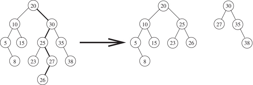
Figure 3.11Splitting a binary search tree with k = 26.
All of the operations described above take O(h) time, where h is the height of the binary search tree. The bounds on the height of a binary tree are derived in Lemma 3.7. It has been shown that when insertions and deletions are made at random, the height of the binary search tree is O(log n) on the average.
Heaps are used to implement priority queues. In a priority queue, the element with highest (or lowest) priority is deleted from the queue, while elements with arbitrary priority are inserted. A data structure that supports these operations is called a max(min) priority queue. Henceforth, in this chapter, we restrict our discussion to a max priority queue. A priority queue can be implemented by a simple, unordered linked list. Insertions can be performed in O(1) time. However, a deletion requires a search for the element with the largest priority followed by its removal. The search requires time linear in the length of the linked list. When a max heap is used, both of these operations can be performed in O(log n) time.
A max heap is a complete binary tree such that for each node, the key value in the node is greater than or equal to the value in its children. Observe that this implies that the root contains the largest value in the tree. Figure 3.12 shows some examples of max heaps.
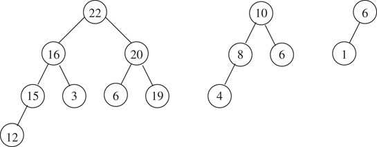
Figure 3.12Max heaps.
We define a class Heap with the following data members.
 private:
   Element *heap;
   int n; // current size of max heap
   int MaxSize; // Maximum allowable size of the heap
The heap is represented using an array (a consequence of the complete binary tree property) which is dynamically allocated.
Suppose that the max heap initially has n elements. After insertion, it will have n + 1 elements. Thus, we need to add a node so that the resulting tree is a complete binary tree with n + 1 nodes. The key to be inserted is initially placed in this new node. However, the key may be larger than its parent resulting in a violation of the max property with its parent. In this case, we swap keys between the two nodes and then repeat the process at the next level. Figure 3.13 demonstrates two cases of an insertion into a max heap.
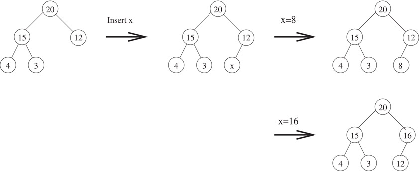
Figure 3.13Insertion into max heaps.
The algorithm is described below. In the worst case, the insertion algorithm moves up the heap from leaf to root spending O(1) time at each level. For a heap with n elements, this takes O(log n) time.
 void MaxHeap::Insert(Element x)
 {
   if (n == MaxSize) {HeapFull(); return;}
   n++;
   for (int i = n; i > 1; i = i/2 ) {
     if (x.key <= heap[i/2].key) break;
     heap[i] = heap[i/2];
   }
   heap[i] = x;
 }
The element to be deleted (i.e., the maximum element in the heap) is removed from the root node. Since the binary tree must be restructured to become a complete binary tree on n − 1 elements, the node in position n is deleted. The element in the deleted node is placed in the root. If this element is less than either of the root’s (at most) two children, there is a violation of the max property. This is fixed by swapping the value in the root with its larger child. The process is repeated at the other levels until there is no violation. Figure 3.14 illustrates deletion from a max heap.
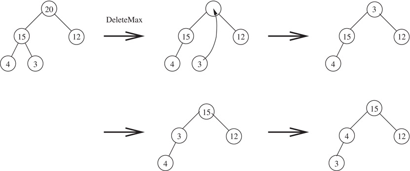
Figure 3.14Deletion from max heaps.
The deletion algorithm is described below. In the worst case, the deletion algorithm moves down the heap from root to leaf spending O(1) time at each level. For a heap with n elements, this takes O(log n) time.
 Element* MaxHeap::DeleteMax(Element& x)
 {
   if (n == 0) {HeapEmpty(); return 0;}
   x = heap[1];
   Element last = heap[n];
   n--;
   for (int i = 1, j = 2; j <= n; i = j, j *= 2) {
     if (j < n)
       if (heap[j].key < heap[j+1].key) j++;
     // j points to the larger child
     if (last.key >= heap[j].key) break;
     heap[i] = heap[j]; // move child up
   }
   heap[i] = last;
   return &x;
 }
Consider the following problem: suppose we have k sequences, each of which is sorted in nondecreasing order, that are to be merged into one sequence in nondecreasing order. This can be achieved by repeatedly transferring the element with the smallest key to an output array. The smallest key has to be found from the leading elements in the k sequences. Ordinarily, this would require k − 1 comparisons for each element transferred. However, with a tournament tree, this can be reduced to log2k comparisons per element.
A winner tree is a complete binary tree in which each node represents the smaller of its two children. The root represents the smallest node in the tree. Figure 3.15 illustrates a winner tree with k = 8 sequences. The winner of the tournament is the value 8 from sequence 0. The winner of the tournament is the smallest key from the 8 sequences and is transferred to an output array. The next element from sequence 0 is now brought into play and a tournament is played to determine the next winner. This is illustrated in Figure 3.16. It is easy to see that the tournament winner can be computed in Θ(log n) time.
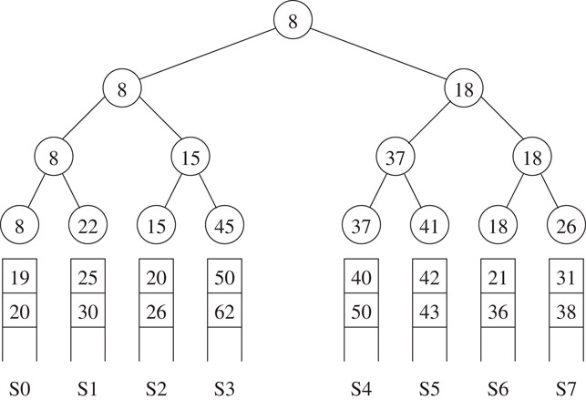
Figure 3.15A winner tree for k = 8. Three keys in each of the eight sequences are shown. For example, sequence 2 consists of 15, 20, and 26.
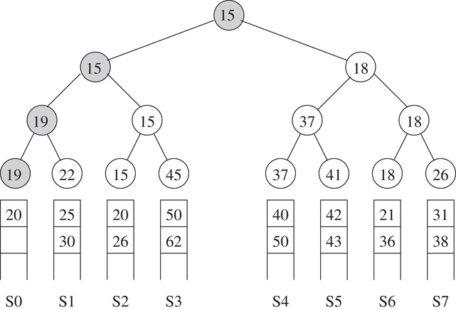
Figure 3.16Winner tree of Figure 3.15 after the next element of sequence 0 plays the tournament. Matches are played at the shaded nodes.
The loser tree is an alternative representation that stores the loser of a match at the corresponding node. The loser tree corresponding to Figure 3.15 is shown in Figure 3.17. An advantage of the loser tree is that to restructure the tree after a winner has been output, it is sufficient to examine nodes on the path from the leaf to the root rather than the siblings of nodes on this path.
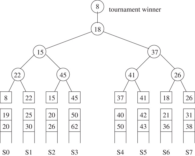
Figure 3.17Loser tree corresponding to the winner tree of Figure 3.15.
The author would like to thank Kun Gao and Mr. U. B. Rao for proofreading this chapter. This work was supported, in part, by the National Science Foundation under grant CCR-9988338.
1.D. Knuth, The Art of Computer Programming, Vol. 1, Fundamental Algorithms, Third edition. Addison Wesley, NY, 1997.
2.T. Cormen, C. Leiserson, R. Rivest, and C. Stein, Introduction to Algorithms, Second edition. McGraw-Hill, New York, NY, 2001.
3.S. Sahni, Data Structures, Algorithms, and Applications in C++, McGraw-Hill, NY, 1998.
4.S. Sahni, Data Structures, Algorithms, and Applications in Java, McGraw-Hill, NY, 2000.
5.R. Sedgewick, Algorithms in C++, Parts 1–4, Third edition. Addison-Wesley, NY, 1998.
6.E. Horowitz, S. Sahni, and D. Mehta, Fundamentals of Data Structures in C++, W. H. Freeman, NY, 1995.
7.D. Stanton and D. White, Constructive Combinatorics, Springer-Verlag, NY, 1986.
*This chapter has been reprinted from first edition of this Handbook, without any content updates.