
Shin-ichi Minato
Hokkaido University
32.4Construction of BDDs from Boolean Expressions
Binary Logic Operation•Complement Edges
32.5Variable Ordering for BDDs
32.7Related Research Activities
Binary decision diagrams (BDDs) are a powerful means for computer processing of Boolean functions because in many cases, with BDDs, smaller memory space is required for storing Boolean functions, and values of functions can be calculated faster than with truth tables or logic expressions. The BDD-based techniques are now used in many application areas in computer science, for example, hardware/software system design, fault analysis of large-scale systems, constraint satisfaction problems, data mining/knowledge discovery, machine learning/classification, bioinformatics, and web data analysis.
Systematic methods for Boolean function manipulation were first studied by Shannon in 1938 [40], who applied Boolean algebra to logic network design. The concept of BDD was devised by Lee in 1959 [22]. Binary decision programs that Lee discussed are essentially BDDs. Then, in 1978, its usefulness for expression Boolean functions was shown by Akers [1]. But since the epoch-making paper by Bryant in 1986 [6], BDD-based methods have been extensively used for many practical applications.
BDD was originally developed for the efficient Boolean function manipulation required in VLSI logic design, but Boolean functions are also used for modeling many kinds of combinatorial problems. Zero-suppressed BDD (ZDD) [29] is a variant of BDD, customized for manipulating “sets of combinations.” ZDDs have been successfully applied not only for VLSI design but also for solving various combinatorial problems, such as constraint satisfaction, frequent pattern mining, and graph enumeration. Recently, BDD and ZDD become more widely known, since Knuth intensively discussed BDD/ZDD-based algorithms in a volume of his book series [19].
Although a quarter of a century has passed since Bryant first put forth his idea, there are still many interesting research topics related to BDD and ZDD. For example, Knuth presented a very fast algorithm “Simpath” [19] to construct a ZDD which represents all the paths connecting two points in a given graph structure. This work is important since it may have many useful applications. Another example of recent activity is to extend BDDs to represent other kinds of discrete structures, such as sequences and permutations. In this context, new variants of BDDs called sequence BDD [22] and πDD [32] have recently been proposed and the scope of BDD-based techniques is now increasing.
In this chapter, we discuss the basic data structures and algorithms for manipulating BDDs. Then we describe the variable ordering problem, which is important for the effective use of BDDs. Finally we give a brief overview of the recent research activities related to BDDs.
From a truth table, we can easily derive the corresponding BDD. For example, the truth table in Figure. 32.1a can be converted into the BDD in Figure. 32.1b. But there are generally many BDDs for a given truth table, that is, the Boolean function expressed by this truth table. For example, all BDDs shown in Figure 32.1c–e represent the Boolean function that the truth table in Figure 32.1a expresses. Here, note that in each of Figures 32.1b–d, the variables appear in the same order and none of them appears more than once in every path from the top node. But in (e), they appear in different orders in different paths. BDDs in Figures 32.1b–d are called ordered BDDs (or OBDDs). But the BDD in Figure 32.1(e) is called an unordered BDD. These BDDs can be reduced into a simple BDD by the following procedure.
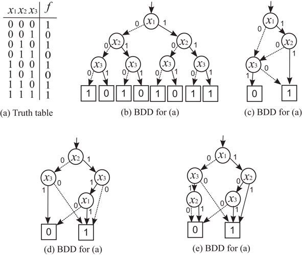
Figure 32.1Truth table and BDDs for .
In a BDD, the top node is called the root that represents the given function f(x1, x2, …, xn). Rectangles that have 1 or 0 inside are called terminal nodes. They are also called 1-terminal and 0-terminal. Other nodes are called nonterminal nodes (or decision nodes) denoted by circles with variables inside. They are also called simply nodes, differentiating themselves from the 0- and 1-terminals. From a node with xi inside, two lines go down. The solid line is called 1-edge, representing xi = 1; and the dotted line is called 0-edge, representing xi = 0.
In an OBDD, the value of the function f can be evaluated by following a path of edges from the root node to one of the terminal nodes. If the nodes in every path from the root node to a terminal node are assigned with variables, x1, x2, …, and xn, in this order, then f can be expressed as follows, according to the Shannon expansion. By branching with respect to x1 from the root node, f(x1, x2, …, xn) can be expanded as follows, where f(0, x2, …, xn) and f(1, x2, …, xn) are functions that the nodes at the low ends of 0-edge and 1-edge from the root represent, respectively:
Then, by branching with respect to x2 from each of the two nodes that f(0, x2, …, xn) and f(1, x2, …, xn) represent, each f(0, x2, …, xn) and f(1, x2, …, xn) can be expanded as follows:
and
and so on.
As we go down from the root node toward the 0- or 1-terminal, more variables of f are set to 0 or 1. Each term excluding xi or in each of these expansions (i.e., f(0, x2, …, xn) and f(1, x2, …, xn) in the first expansion, f(0, 0, …, xn) and f(0, 1, …, xn) in the second expansion, etc.), are called cofactors. Each node at the low ends of 0-edge and 1-edge from a node in an OBDD represents cofactors of the Shannon expansion of the Boolean function at the node, from which these 0-edge and 1-edge come down.
Procedure 32.1
Reduction of a BDD
1.For the given BDD, apply the following steps in any order.
a.Sharing equivalent nodes: If two nodes va and vb, that represent the same variable xi, branch to the same nodes in a lower level for each of xi = 0 and xi = 1, then combine them into one node that still represents variable xi (see Figure 32.2). Similarly, two terminal nodes with the same value, 0 or 1, are merged into one terminal node with the same original value.
b.Deleting redundant nodes: If a node that represents a variable xi branches to the same node in a lower level for both xi = 0 and xi = 1, then that node is deleted, and the edges that come down to the former are extended to the latter (see Figure 32.3).
2.When we cannot apply any step after repeatedly applying these steps (a) and (b), the reduced ordered BDD (i.e., ROBDD) or simply called the reduced BDD is obtained for the given function.

Figure 32.2Step 1(a) of Procedure 32.1 (node sharing rule).

Figure 32.3Step 1(b) of Procedure 32.1 (node deletion rule).
In Figure 32.4, we show an example of applying the BDD reduction rules, starting from the same BDD shown in Figure 32.1b.

Figure 32.4An example of applying node reduction rules.
Theorem 32.1
Any Boolean function has a unique reduced ordered BDD and any other ordered BDD for the function in the same variable order (i.e., not reduced) has more nodes.
According to this theorem, the ROBDD is unique for a given Boolean function when the order of the variables is fixed. Thus ROBDDs give canonical forms for Boolean functions. This property is very important to practical applications, as we can easily check the equivalence of two Boolean functions by only checking the isomorphism of their ROBDDs. Henceforth in this chapter, ROBDDs will be referred to as BDDs for the sake of simplicity.
It is known that a BDD for an n-variable function requires an exponentially increasing memory space in the worst cases, as n increases [6]. However, the size of memory space for the BDD varies with the types of functions, unlike truth tables which always require memory space proportional to 2n. But many Boolean functions that we encounter in design practice can be represented in BDDs without large memory space. This is an attractive feature of BDDs. Figure 32.5 shows the BDDs representing typical functions, AND, OR, and the parity function with three input variables. The parity function for n variables, x1 ⊕ x2 ⊕ ··· ⊕ xn, can be represented in the BDD of 2(n − 1) + decision nodes and 2 terminals, whereas, if a truth table or a logic expression is used, the size increases exponentially as n increases.
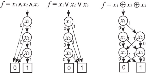
Figure 32.5BDDs for typical Boolean functions.
A set of BDDs representing many functions can be obtained into a graph that consists of BDDs sharing subgraphs among them, as shown in Figure 32.6. This idea saves time and space for duplicating isomorphic BDDs. By sharing all the isomorphic subgraphs completely, no two nodes that express the same function coexist in the graph. We call it shared BDDs [29] or multirooted BDDs. In a shared BDD, no two root nodes express the same function.

Figure 32.6A shared BDD.
Shared BDDs are now widely used and those algorithms are more concise than ordinary BDDs. In the remainder of this chapter, we deal with shared BDD only.
In a typical realization of a BDD manipulator, all the nodes are stored in a single table in the main memory of the computer. Figure 32.7 is a simple example of realization for the shared BDD shown in Figure 32.6. Each node has three basic attributes: input variable and the next nodes accessed by 0- and 1-edges. Also, 0- and 1-terminals are first allocated in the table as special nodes. The other nonterminal nodes are created one by one during the execution of logic operations.

Figure 32.7Table-based realization of a shared BDD.
Before creating a new node, we check the reduction rules of Procedure 32.1. If the 0- and 1-edges go to the same next node (Step 1(b) of Procedure 32.1) or if an equivalent node already exists (Step 1(a) of Procedure 32.1), then we do not create a new node but simply copy the pointer to the existing node. To find an equivalent node, we check a table which displays all the existing nodes. The hash table technique is very effective to accelerate this checking. (It can be done in a constant time for any large-scale BDDs, unless the table overflows in main memories.) The procedure to get a decision node is summarized as follows.
Procedure 32.2
GetNode(variable x, 0-edge to f0, 1-edge to f1)
1.If (f0 = f1), just return f0.
2.Check the hash table, and if an equivalent node f is found, then return f.
3.If no more available space, return by memory overflow error, otherwise, create a new node f with the attribute (x, f0, f1) and return f.
In manipulating BDDs for practical applications, we sometimes generate many intermediate (or temporary) BDDs. It is important for memory efficiency to delete such unnecessary BDDs. In order to determine the necessity of the nodes, a reference counter is attached to each node, which shows the number of incoming edges to the node.
In a typical implementation, the BDD manipulator consumes 30–40 bytes of memory for each node. Today, there are personal computers with 32 or 64 Gbytes of memory, and those facilitate us to generate BDDs containing as many as billions of nodes. However, the BDDs still grow beyond the memory capacity in some practical applications.
32.4Construction of BDDs from Boolean Expressions
Procedure 32.1 shows a way of constructing compact BDDs from the truth table for a function f of n variables. This procedure, however, is not efficient because the size of its initial BDD is always of the order of 2n, even for a very simple function. In order to avoid this problem, Bryant [6] presented a method of constructing BDDs by applying a sequence of logic operations in a Boolean expression.
Figure 32.8 summarizes the list of primitive operations for constructing and manipulating BDDs. Using these operations, we can construct BDDs for an arbitrary Boolean expression. This method is generally far more efficient than that based on a truth table.
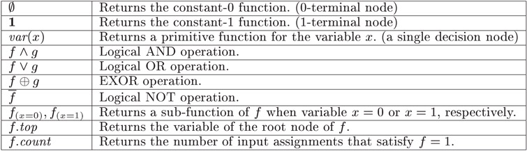
Figure 32.8Primitive operations for BDD manipulation.
Figure 32.9 shows a simple example of constructing a BDD for . First, trivial BDDs for x1, x2, and x3 are created in Figure 32.9a. Next, applying the AND operation between x1 and x2, the BDD for (x1 ∧ x2) is then generated. The BDD for can be derived by applying NOT operation to the BDD for x3. Then the BDD for the entire expression is obtained as the result of the OR operation between (x1 ∧ x2) and . After deleting the nodes that are not on the paths from the root node for f toward the 0- or 1-terminal, the final BDD is obtained as shown in Figure 32.9b.

Figure 32.9Constructing BDDs for .
In the following, we describe a formal procedure for generating a BDD by applying binary logic operation between two BDDs.
Suppose we perform a binary operation between two functions f and g, and this operation is denoted by f○g, where ○ is one of OR, AND, EXOR, and others. Then by the Shannon expansion of a function explained previously, f○g can be expanded as follows:
with respect to variable xi, which is the variable of the node that is in the highest level among all the nodes in f and g. This expansion creates a new decision node with the variable xi having 0- and 1-edges pointing to the two nodes generated by suboperations and . This formula means that the operation can be expanded to the two sub-operations and . Repeating this expansion recursively for all the variables, as we go down toward the 0- or 1-terminal, we will have eventually trivial operations, such as f · 1 = f, f ⊕ f = 0, and 0 ∨ g = g, and the result is obtained.
The procedure of constructing h ○ f°g is summarized as follows. Here f0 and f1 are the BDDs pointed to by the 0- and 1-edges from the root node of f.
Procedure 32.3
Construction of a BDD for Function h ○ f°g, given BDDs for f and g
1.When f or g is a constant or when f = g:
return a result according to the type of the operation
(e.g., f · 1 = f, f ⊕ f = 0, 0 ∨ g = g)
2.If f.top and g.top are identical:
; ;
3.If f.top is higher than g.top:
; ;
4.If f.top is lower than g.top:
compute similarly to 3 by exchanging f and g.
As mentioned in the previous section, we check the BDD reduction rules before creating a new nodes to avoid duplication of the equivalent nodes.
Figure 32.10a shows an example of execution. When we perform the operation between the node N8 and N7, the procedure is broken down into the binary tree, as shown in Figure 32.10b. We usually execute the procedure calls according to this tree structure in a depth-first manner, and it may require an exponential time for the number of variables. However, some of these subtrees may be redundant; for instance, the operations of N4 − N2 and N2 − N3 appear more than once. We can accelerate the procedure by using a hash-based cache that memorizes the results of recent operations. We call it operation cache. By referring to the operation cache before every recursive call, we can avoid duplicate executions for equivalent suboperations. This technique enables the binary logic operations to be executed in a time almost proportional to the total size of BDDs for f, g, and h. (For detailed discussions, refer the article [45].)

Figure 32.10Procedural structure of generating BDDs for h = f ∨ g.
It is too memory-consuming to keep all the operation results for any different pairs of BDD nodes, therefore, we usually prepare a limited size of the operation cache. If some of operation results have been lost, then some number of redundant suboperations may be called, but anyway, the correct BDD can be constructed by applying BDD reduction rules. The size of operation cache has a significant influence to the performance of BDD manipulation. If the cache size is insufficient, the more redundant procedure calls increase, the more results are overwritten, and the total execution time grows rapidly. Usually we set up the cache size empirically, for instance, it is proportional to the total number of BDD nodes created in the system.
A BDD for , the complement of f, has a form similar to that of the BDD for f: just the 0- and the 1-terminals are exchanged. Complemental BDDs contain the same number of nodes, in contrast to the conjunctive/disjunctive normal forms (CNFs/DNFs), which sometimes suffer an exponential increase of the data size.
By using binary logic operation (f ⊕ 1), we can generate a BDD for in a linear time for the BDD size. However, the operation is improved to a constant time by using complemented edges. The complemented edge is a technique to reduce computation time and space for BDDs by using attributed edges that indicate to complement the function of the subgraph pointed to by the edge, as shown in Figure 32.11a. This idea was first shown by Akers [1] and later discussed by Madre et al. [23]. Today, this technique is commonly used in most of BDD packages. The use of complement edges brings the following outstanding merits:
•The BDD size is reduced by up to half.
•NOT operation can be performed in a constant time.
•Binary logic operations are sped up by applying the rules, such as , and .

Figure 32.11Complement edges.
Use of complement edges may break the uniqueness of BDDs. Therefore, we have to put the two rules as illustrated in Figure 32.11b:
•Using the 0-terminal only
•Not using a complement edges at the 0-edge of any node (i.e., it can be used at 1-edge only). If necessary, the complement edges can be carried over to higher nodes.
32.5Variable Ordering for BDDs
BDDs are a canonical representation of Boolean functions under a fixed order of input variables. A change of the order of variables, however, may yield different BDDs of significantly different sizes for the same function. The effect of variable ordering depends on Boolean functions, sometimes dramatically changing the size of BDDs. Variable ordering is an important problem in using BDDs.
It is generally very time-consuming to find the best order. Friedman et al. presented an algorithm [15] of O(n23n) time based on dynamic programming, where n is the number of variables. Although this algorithm has been improved [12], existing methods are limited to run on the small size of BDDs with up to about 20 variables. This problem is known as an NP-complete problem [44], and it would be difficult to find the best order for larger problems in reasonably short processing time. However, if we can find a fairly good order, it is useful for practical applications. There are many research works on heuristic methods of variable ordering.
Empirically, the following properties are known on the variable ordering.
1.Closely-related variables:
Variables that are in close relationship in a Boolean expression should be close in variable order. For example, the Boolean function of AND–OR two-level logic has a BDD with 2n decision nodes in the best order as shown for n = 4 in Figure 32.12a, while it needs (2(n+1) − 2) nodes in the worst order, as shown in Figure 32.12b.
2.Influential variables:
The variables that greatly influence the nature of a function should be at higher position. For example, the 8-to-1 data selector shown in Figure 32.13a can be represented by a linear size of BDD when the three control inputs are ordered high, but when the order is reversed, it becomes of exponentially increasing size as the number of variables increases, as shown in Figure 32.13b.

Figure 32.12BDDs for (x1 ∧ x2) ∨ (x3 ∧ x4) ∨ (x5 ∧ x6) ∨ (x7 ∧ x8).

Figure 32.13BDDs for 8-to-1 data selector.
Based on empirical rules like this, Fujita et al. [13] and Malik et al. [25] presented methods; in these methods, an output of the given logic networks is reached, traversing in a depth-first manner, then an input variable that can be reached by going back toward the inputs of the network is placed at highest position in variable ordering. Minato [33] devised another heuristic method based on a weight propagation procedure for the given logic network. Butler et al. [5] proposed another heuristic based on a measure which uses not only the connection configuration of the network but also the output functions of the network. These methods probably find a good order before generating BDDs. They find good orders in many cases, but there is no method that is always effective to a given network.
Another approach reduces the size of BDDs by reordering input variables. A greedy local exchange (swapping adjacent variables) method was developed by Fujita et al. [14]. Minato [28] presented another reordering method which measures the width of BDDs as a cost function. In many cases, these methods find a fairly good order using no additional information. A drawback of the approach of these methods is that they cannot start if an initial BDD is too large.
One remarkable work is dynamic variable ordering, presented by Rudell [39]. In this technique, the BDD manipulation system itself determines and maintains the variable order. Every time the BDD grow to a certain size, the reordering process is invoked automatically. This method is very effective in terms of the reduction of BDD size, although it sometimes takes a long computation time.
Unfortunately, there are some hard examples where variable ordering is powerless. For example, Bryant [6] proved that an n-bit multiplier function requires an exponentially increasing number of BDD nodes for any variable order, as n increases. From a theoretical viewpoint, the total number of different n-input Boolean functions is , and the number of permutation of n variables is only n!, which is much less than . This means that after variable ordering, the variation of Boolean functions is still a double exponential number, and we still need exponential size of data structure in the worst case to distinguish all the functions. Thus we expect that the variable ordering methods would not be effective for generally randomized functions. However, empirically we can say that, for many practical functions, the variable ordering methods are very useful for generating a small size of BDDs in a reasonably short time.
BDDs are originally developed for handling Boolean function data, however, they can also be used for implicit representation of combinatorial sets. Here we call set of combinations for a set of elements each of which is a combination out of n items. This data model often appears in real-life problems, such as combinations of switching devices, Boolean item sets in the database, and combinatorial sets of edges or nodes in the graph data model.
A set of combinations can be mapped into Boolean space of n input variables. If we choose any one combination of items, a Boolean function determines whether the combination is included in the set of combinations. Such Boolean functions are called characteristic functions. The set operations such as union, intersection, and difference can be performed by logic operations on characteristic functions. Figure 32.14 shows an example of the Boolean function corresponding to the set of combinations F = {ac, b}.

Figure 32.14Correspondence of Boolean function and set of combinations.
By using BDDs for characteristic functions, we can manipulate sets of combinations efficiently. They can be generated and manipulated within a time roughly proportional to the BDD size. When we handle many combinations including similar patterns (subcombinations), BDDs are greatly reduced by node sharing effect, and sometimes an exponential reduction benefit can be obtained.
Zero-suppressed BDD (ZDD or ZBDD) [29,30] is a special type of BDD for efficient manipulation of sets of combinations. Figure 32.15 shows an example of BDD and ZDD for the same set of combinations F = {ac, b}.

Figure 32.15BDD and ZDD for the same set of combinations F = ac, b.
ZDDs are based on the following special reduction rules:
•Delete all nodes whose 1-edge directly points to the 0-terminal node, and jump through to the 0-edge’s destination, as shown in Figure 32.16
•Share equivalent nodes as well as ordinary BDDs.

Figure 32.16Reduction rule for ZDDs.
Notice that we do not delete the nodes whose two edges point to the same node, which used to be deleted by the original rule. The zero-suppressed deletion rule is asymmetric for the two edges, as we do not delete the nodes whose 0-edge points to a terminal node. It is proved that ZDDs also give canonical forms as well as ordinary BDDs under a fixed variable ordering.
Here we summarize the features of ZDDs.
•In ZDDs, the nodes of irrelevant items (never chosen in any combination) are automatically deleted by ZDD reduction rule. In ordinary BDDs, irrelevant nodes still remain and they may cause unnecessary computation.
•ZDDs are especially effective for representing sparse combinations. If the average appearance ratio of each item is 1%, ZDDs are possibly up to 100 times more compact than ordinary BDDs. Such situations often appear in real-life problems, for example, in a supermarket, the number of items in a customer’s basket is usually much less than the number of all the items displayed.
•Each path from the root node to the 1-terminal node corresponds to each combination in the set. Namely, the number of such paths in the ZDD equals to the number of combinations in the set. In ordinary BDDs, this property does not always hold.
•When no equivalent nodes exist in a ZDD, that is the worst case, the ZDD structure explicitly stores all items in all combinations, as well as using an explicit linear linked list data structure. Namely, (the order of) ZDD size never exceeds the explicit representation. An example is shown in Figure 32.17. If more nodes are shared, the ZDD is more compact than linear list. Ordinary BDDs have larger overhead to represent sparser combinations while ZDDs have no such overhead.

Figure 32.17Explicit representation with ZDD.
Figure 32.18 shows an example of constructing ZDDs. As well as ordinary BDDs, any set of combinations can be generated by a sequence of primitive operations. Figure 32.19 summarizes most of the primitive operations of the ZDDs. In these operations, ∅, {λ}, and F.top can be obtained in constant time. Here λ means a null combination. F.offset(x), F.onset(x), and F.change(x) operations require a constant time if x is the top variable of F, otherwise they require a time linear in the number of ZDD nodes located at a higher position than x. The union, intersection, and difference operations can be performed in a time that is linear in the size of the ZDDs in many practical cases.
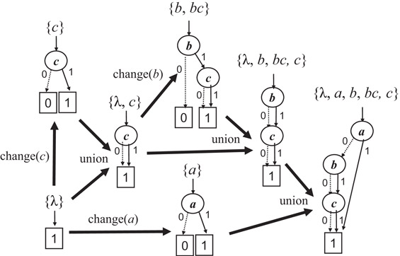
Figure 32.18Example of constructing ZDDs.

Figure 32.19Primitive ZDD operations.
The last three operations in the table constitute an interesting algebra for sets of combinations with multiplication and division. Knuth has been inspired by this idea and has developed more various algebraic operations, such as F ⊓ G, F ⊔ G, F ⊞ G, F ↗ G, F ↘ G, F↑, and F↓. He called these ZDD-based operations a “Family Algebra” in the recent fascicle of his book series [19].
The original BDD was developed for VLSI logic design, but ZDD is now recognized as the most important variant of BDD, and is widely used in various kinds of problems in computer science [10,17,21,35].
32.7Related Research Activities
In the last section of this chapter, we present an overview of research activities related to BDDs and ZDDs. Of course, it is impossible to cover all the research activities in this limited space, so there may be many other interesting topics which are not shown here.
In 1986, Bryant proposed the algorithm called “Apply” [6]. It was the origin of much work on the use of BDDs as modern data structures and algorithms for efficient Boolean function manipulation. Just after Bryant’s paper, implementation techniques for the BDD manipulation, such as hash-table operations and memory management techniques, emerged [4,33]. A BDD is a unique representation of a given Boolean function. However, if the order of input variables is changed, a different BDD is obtained for what is essentially the same Boolean function. Since the size of BDDs greatly depends on the order of input variables, variable ordering methods were intensively developed in the early days [12,14,39,44]. Those practical techniques were implemented in a software library called “BDD package.” Currently, several academic groups provide such packages as open software (e.g., CUDD package [42]).
At first, BDDs were applied to equivalence checking of logic circuits [7,13,25] and logic optimization [26] in VLSI logic design. Next, BDD-based symbolic manipulation techniques were combined with the already known theory of model checking. It was really a breakthrough that formal verification becomes possible for some practical sizes of sequential machines [3,27]. After that, many researchers became involved with formal hardware verification using BDDs, and Clarke received the Turing Award in 2008 for this work. In addition, the BDD-based symbolic model checking method led to the idea of bounded model checking using SAT solvers [2,37,42]. These research produced many practical applications of SAT solvers that are widely utilized today.
ZDDs [29] deal with sets of combinations, representing a model that is different from Boolean functions. However, the original motivation of developing ZDDs was also for VLSI logic design. ZDDs were first used for manipulating very large-scale logic expressions with an AND–OR two-level structure (also called DNF or CNF), namely, representing a set including very large number of combinations of input variables. Sets of combinations often appear not only in VLSI logic design area but also in various areas of computer science. It is known that ZDDs are effective for handling many kinds of constraint satisfaction problems in graph theory and combinatorics [10,38].
After the enthusiastic research activities in 1990s, one can observe a relatively inactive period between 1999 and 2005. We may call these years the “Winter of BDDs.” On that time, most basic implementation techniques had been matured, and BDD applications to VLSI design tools seemed to be almost exhausted. So, many researchers moved from BDD-related work to other research areas, such as actual VLSI chip design issues or SAT-based problem solving.
However, after about 2005, many people understood that BDDs/ZDDs are useful not only for VLSI logic design but also in various other areas, and then BDD-related research activity was revived. For example, we can see some applications to data mining [21,31,36], Bayesian network and probabilistic inference models [17,35], and game theory [43]. More recently, new types of BDD variants, which have not been considered before, have been proposed. Sequence BDDs [22] represent sets of strings or sequences, and πDD [32] represent sets of permutations.
Synchronizing with this new movement, the BDD section of Knuth’s book was published [19]. As Knuth presented the potential for wide-ranging applications of BDDs and ZDDs, these data structures and algorithms were recognized as fundamental techniques for whole fields of information science. In particular, his book includes the “Simpath” algorithm which constructs a ZDD representing all the connecting paths between two points in a given graph structure, and a surprisingly fast program is provided for public use on his web page. Experimental results suggest that this algorithm is not just an exercise but is the most efficient method using current technology. Based on this method, the author’s research group is now developing extended and generalized algorithms, called “Frontier-based methods,” for efficiently enumerating and indexing various kinds of discrete structures [16,18,46].
As the background of this resurgence and new generation applications, we should note the great progress of the computer hardware system, especially the increase of main memory capacity. Actually, in the early days of using BDDs in 1990s, there was some literature on applications for intelligent information processing. Madre and Coudert proposed a TMS (Truth Maintenance System) using BDDs for automatic logic inference and reasoning [24]. A method of probabilistic risk analysis for large industrial plants was also considered [9]. Coudert also proposed a fast method of constructing BDDs to represent prime sets (minimal support sets) for satisfying Boolean functions [8], which is a basic operation for logic inference. However, at that time, the main memory capacities of high specification computers were only 10–100 megabytes, about 10,000 times smaller than those available today, and thus, only small BDDs could be generated.
In the VLSI design process, the usual approach was that the whole circuit was divided into a number of small submodules, and each submodule was designed individually by hand. So, it was natural that the BDD-based design tools are used for the sufficiently small submodules which could be handled with a limited main memory capacity. With the progress of computer hardware performance, BDD-based methods could gradually be applied to larger submodule. On the other hand, in the applications of data mining or knowledge processing, the input data were stored on a very large hard disks. The processor loaded a small fragment of data from the hard disk into the main memory and executed some meaningful operations on the data in the main memory, then the processed data was saved with the original data on the hard disk. Such procedures were common, but it was very difficult to apply BDD-based methods to hard disk data. After 2000, computers’ main memory capacity grew rapidly, and in many practical cases, all the input data can be stored in the main memory. Thus many kinds of in-memory algorithms could be actively studied for data processing applications. The BDD/ZDD algorithm is a typical instance of such in-memory techniques.
In view of the above technical background, most research on BDDs/ZDDs after the winter period is not just about remaking old technologies. It also compares classical and well-known efficient methods (such as suffix trees, string matching, and frequent pattern mining) with the BDD/ZDD-based methods, in order to propose combined or improved techniques to obtain the current best performance. For example, Darwiche, who is a well-known researcher in data structures of probabilistic inference models, is very interested in the techniques of BDDs, and he recently proposed a new data structure, the SDD (Sentential Decision Diagram) [11], to combine BDDs with the classical data structures of knowledge databases. As shown in this example, we had better collaborate with many researchers in various fields of information science to import the current best known techniques into BDD/ZDD related work, and then we may develop more efficient new data structures and algorithms for discrete structure manipulation.
This work was supported, in part, by JST ERATO Minato Discrete Structure Manipulation System Project and by JSPS KAKENHI Grant Number 15H05711. A part of this article is based on my old work [34] coauthored with the late Professor Saburo Muroga.
1.S. B. Akers. Binary decision diagrams. IEEE Transactions on Computers, C-27(6): 509–516, 1978.
2.A. Biere, A. Cimatti, E. M. Clarke, M. Fujita, and Y. Zhu. Symbolic model checking using sat procedures instead of BDDs. In Proceedings of the 36th Annual ACM/IEEE Design Automation Conference, DAC’99, pages 317–320, New Orleans, LA, 1999. ACM.
3.J. R. Burch, E. M. Clarke, K. L. McMillan, and David L. Dill. Sequential circuit verification using symbolic model checking. In Proceedings of the 27th ACM/IEEE Design Automation Conference, DAC’90, pages 46–51, Orland, FL, 1990. IEEE Computer Society Press.
4.K. S. Brace, R. L. Rudell, and R. E. Bryant. Efficient implementation of a BDD package. In Proceedings of the 27th ACM/IEEE Design Automation Conference, DAC’90, pages 40–45, Orland, FL, 1990. IEEE Computer Society Press.
5.K. M. Butler, D. E. Ross, R. Kapur, and M. R. Mercer. Heuristics to compute variable orderings for efficient manipulation of ordered binary decision diagrams, In Proceedings of 28th ACM/IEEE Design Automation Conference (DAC’88), pages 417–420, San Francisco, CA, June 1991.
6.R. E. Bryant. Graph-based algorithms for Boolean function manipulation. IEEE Transactions on Computers, C-35(8):677–691, 1986.
7.O. Coudert and J. C. Madre. A unified framework for the formal verification of sequential circuits. In Proceedings of IEEE International Conference on Computer-Aided Design (ICCAD’90), pages 126–129, Santa Clara, CA, 1990. IEEE Computer Society Press.
8.O. Coudert and J. C. Madre. Implicit and incremental computation of primes and essential primes of Boolean functions. In Proceedings of the 29th ACM/IEEE Design Automation Conference, DAC’92, pages 36–39, Anaheim, CA, 1992. IEEE Computer Society Press.
9.O. Coudert and J. C. Madre. Towards an interactive fault tree analyser. In Proceedings of IASTED International Conference on Reliability, Quality Control and Risk Assessment, Washington D.C., 1992.
10.O. Coudert. Solving graph optimization problems with ZBDDs. In Proceedings of ACM/IEEE European Design and Test Conference (ED&TC’97), pages 224–228, Munchen, Germany, 1997. IEEE Computer Society Press.
11.A. Darwiche. SDD: A new canonical representation of propositional knowledge bases. In Proceedings of 22nd International Joint Conference of Artificial Intelligence (IJCAI’2011), pages 819–826, Barcelona, Spain, 2011. AAAI Press.
12.R. Drechsler, N. Drechsler, and W. Günther. Fast exact minimization of BDDs. In Proceedings of the 35th Annual Design Automation Conference, DAC’98, pages 200–205, San Francisco, CA, 1998. ACM.
13.M. Fujita, H. Fujisawa, and N. Kawato. Evaluation and implementation of boolean comparison method based on binary decision diagrams. In Proceedings of IEEE International Conference on Computer-Aided Design (ICCAD’88), pages 2–5, Santa Clara, CA, 1988. IEEE Computer Society Press.
14.M. Fujita, Y. Matsunaga, and T. Kakuda. On variable ordering of binary decision diagrams for the application of multi-level logic synthesis. In Proceedings of the Conference on European Design Automation, EURO-DAC’91, pages 50–54, Amsterdam, Netherlands, 1991. IEEE Computer Society Press.
15.S. J. Friedman and K. J. Supowit. Finding the optimal variable ordering for binary decision diagrams, In Proceedings of the 24th ACM/IEEE Design Automation Conference, DAC’87, Miami Beach, FL, pages 348–356, 1987. ACM.
16.H. Iwashita, J. Kawahara, and S. Minato. ZDD-based computation of the number of paths in a graph. Hokkaido University, Division of Computer Science, TCS Technical Reports, TCS-TR-A-10-60, 2012.
17.M. Ishihata, Y. Kameya, T. Sato, and S. Minato. Propositionalizing the EM algorithm by BDDs. In Proceedings of 18th International Conference on Inductive Logic Programming (ILP’2008), Prague, Czech Republic, 2008. Springer.
18.T. Inoue, K. Takano, T. Watanabe, J. Kawahara, R. Yoshinaka, A. Kishimoto, K. Tsuda, S. Minato, and Y. Hayashi. Loss minimization of power distribution networks with guaranteed error. Hokkaido University, Division of Computer Science, TCS Technical Reports, TCS-TR-A-10-59, 2012.
19.D.E. Knuth. Bitwise Tricks & Techniques; Binary Decision Diagrams, volume 4, fascicle 1. Addison-Wesley, Boston, MA, 2009.
20.C. Y. Lee. Representation of switching circuits by binary-decision programs. Bell System Technical Journal, 38(4):985–999, 7 1959.
21.E. Loekit, J Bailey. Fast mining of high dimensional expressive contrast patterns using zero-suppressed binary decision diagrams. In Proceedings of the Twelfth ACM SIGKDD International Conference on Knowledge Discovery and Data Mining (KDD’2006), pages 307–316, Philadelphia, PA, 2006. ACM.
22.E. Loekito, J. Bailey, and J. Pei. A binary decision diagram based approach for mining frequent subsequences. Knowledge and Information Systems, 24(2):235–268, 2010.
23.J. C. Madre and J. P. Billon. Proving circuit correctness using formal comparison between expected and extracted behaviour. In Proceedings of the 25th ACM/IEEE Design Automation Conference (DAC’88), pages 205–210, Anaheim, CA, 1988. IEEE Computer Sciety Press.
24.J. C. Madre and O. Coudert A logically complete reasoning maintenance system based on a logical constraint solver. In Proceedings of the 12th International Joint Conference on Artificial Intelligence—Volume 1, pages 294–299, San Francisco, CA, 1991. Morgan Kaufmann Publishers Inc.
25.S. Malik, A. Wang, R. K. Brayton, and A. S.- Vincentelli. Logic verification using binary decision diagrams in a logic synthesis environment. In Proceedings of the IEEE International Conference on Computer-Aided Design (ICCAD’88), pages 6–9, Santa Clara, CA, 1988. IEEE Computer Society Press.
26.Y. Matsunaga, M Fujita. Multi-level logic optimization using binary decision diagrams. In Proceedings of the IEEE International Conference on Computer-Aided Design (ICCAD’89), pages 556–559, Santa Clara, CA, 1989. IEEE Computer Society Press.
27.K. L. McMillan. Symbolic Model Checking. Kluwer Academic Publishers, 1993.
28.S. Minato. Minimum-width method of variable ordering for binary decision diagrams. IEICE Transactions on Fundamentals, E75-A(3): 392–399, 1992.
29.S. Minato. Zero-suppressed BDDs for set manipulation in combinatorial problems. In Proceedings of the 30th ACM/IEEE Design Automation Conference (DAC’93), pages 272–277, Dallas, TX, 1993. ACM.
30.S. Minato. Zero-suppressed BDDs and their applications. International Journal on Software Tools for Technology Transfer, 3:156–170, Springer, Berlin/Heidelberg.
31.S. Minato. VSOP (valued-sum-of-products) calculator for knowledge processing based on zero-suppressed BDDs. In K. P.SEP Jantke, A. Lunzer, N. Spyratos, and Y. Tanaka, editors, Federation over the Web, volume 3847 of Lecture Notes in Computer Science, pages 40–58. Springer, Berlin/Heidelberg, 2006.
32.S. Minato. πDD: A new decision diagram for efficient problem solving in permutation space. In K. A. Sakallah and L. Simon, editors, Theory and Applications of Satisfiability Testing—SAT 2011, volume 6695 of Lecture Notes in Computer Science, pages 90–104. Springer, Berlin/Heidelberg, 2011.
33.S. Minato, N. Ishiura, and S. Yajima. Shared binary decision diagram with attributed edges for efficient Boolean function manipulation. In Proceedings of 27th ACM/IEEE Design Automation Conference, pages 52–57, Orlando, FL, 1990. IEEE Computer Society Press.
34.S. Minato and S. Muroga. Binary decision diagrams. In W.-K. Chen, editor, The VLSI Handbook, chapter 26, pages 26.1–26.14. CRC/IEEE Press, 1999.
35.S. Minato, K. Satoh, and T. Sato. Compiling Bayesian networks by symbolic probability calculation based on zero-suppressed BDDs, In Proceedings of 20th International Joint Conference of Artificial Intelligence (IJCAI’2007), pages 2550–2555, Hyderabad, India, 2007, AAAI Press. 2007.
36.S. Minato, T. Uno, and H. Arimura. LCM over ZBDDs: Fast generation of very large-scale frequent itemsets using a compact graph-based representation. In T. Washio, E. Suzuki, K. Ting, and A. Inokuchi, editors, Advances in Knowledge Discovery and Data Mining, volume 5012 of Lecture Notes in Computer Science, pages 234–246. Springer, Berlin/Heidelberg, 2008.
37.M. W. Moskewicz, C. F. Madigan, Y. Zhao, L. Zhang, and S. Malik. Chaff: Engineering an efficient sat solver, In Proceedings of the 38th Annual Design Automation Conference, DAC’01, pages 530–535, Las Vegas, NV, 2001. ACM.
38.H. Okuno, S. Minato, and H. Isozaki. On the properties of combination set operations. Information Processing Letters, 66:195–199, 1998. Elsevier.
39.R. Rudell. Dynamic variable ordering for ordered binary decision diagrams. In Proceedings of the 1993 IEEE International Conference on Computer-Aided Design, ICCAD’93, pages 42–47, Santa Clara, CA, 1993. IEEE Computer Society Press.
40.C.E. Shannon. A symbolic analysis of relay and switching circuits. Transactions of the American Institute of Electrical Engineers, 57(12):713–723, 1938.
41.F. Somenzi. Cudd: Cu decision diagram package, 1997. http://vlsi.colorado.edu/fabio/CUDD/.
42.J. P. M. Silva, and K. A. Sakallah. Grasp—A new search algorithm for satisfiability, In Proceedings of the IEEE/ACM International Conference on Computer-Aided Design (ICCAD’96), pages 220–227, San Jose, CA, 1996. IEEE Computer Society Press/ACM.
43.Y. Sakurai, S. Ueda, A. Iwasaki, S. Minato, and M. Yokoo. A compact representation scheme of coalitional games based on multi-terminal zero-suppressed binary decision diagrams. In D. Kinny, J-j. Hsu, G. Governatori, and A. K. Ghose, editors, Agents in Principle, Agents in Practice, volume 7047 of Lecture Notes in Computer Science, pages 4–18. Springer, Berlin/Heidelberg, 2011.
44.S. Tani, K. Hamaguchi, and S. Yajima. The complexity of the optimal variable ordering problems of shared binary decision diagrams. In K. W. Ng, P. Raghavan, N. V. Balasubramanian, and F. Y. L. Chin, editors, Algorithms and Computation, volume 762 of Lecture Notes in Computer Science, pages 389–398. Springer, Berlin/Heidelberg, 1993.
45.R. Yoshinaka, J. Kawahara, S. Denzumi, H.SEP Arimura, and S. Minato. Counterexamples to the long-standing conjecture on the complexity of BDD binary operations. Information Processing Letters, 112(16): 636–640, 2012. Elsevier.
46.R. Yoshinaka, T. Saitoh, J. Kawahara, K. Tsuruma, H.SEP Iwashita, and S. Minato. Finding all solutions and instances of numberlink and slitherlink by ZDDs. Algorithms, 5(2):176–213, 2012. Elsevier.