
Haim Kaplan
Tel Aviv University
33.2Algorithmic Applications of Persistent Data Structures
33.3General Techniques for Making Data Structures Persistent
The Fat Node Method•Node Copying and Node Splitting•Handling Arrays•Making Data Structures Confluently Persistent
33.4Making Specific Data Structures More Efficient
Redundant Binary Counters•Persistent Deques
33.5Concluding Remarks and Open Questions
Think of the initial configuration of a data structure as version zero, and of every subsequent update operation as generating a new version of the data structure. Then a data structure is called persistent if it supports access to all versions and it is called ephemeral otherwise. The data structure is partially persistent if all versions can be accessed but only the newest version can be modified. The structure is fully persistent if every version can be both accessed and modified. The data structure is confluently persistent if it is fully persistent and has an update operation which combines more than one version. Let the version graph be a directed graph where each node corresponds to a version and there is an edge from node V1 to a node V2 if and only of V2 was created by an update operation to V1. For partially persistent data structure the version graph is a path; for fully persistent data structure the version graph is a tree; and for confluently persistent data structure the version graph is a directed acyclic graph (DAG).
A notion related to persistence is that of purely functional data structures. (See Chapter 41 by Okasaki in this handbook.) A purely functional data structure is a data structure that can be implemented without using an assignment operation at all (say using just the functions car, cdr, and cons, of pure lisp). Such a data structure is automatically persistent. The converse, however, is not true. There are data structures which are persistent and perform assignments.
Since the seminal paper of Driscoll, Sarnak, Sleator, and Tarjan (DSST) [1], and over the past fifteen years, there has been considerable development of persistent data structures. Persistent data structures have important applications in various areas such as functional programming, computational geometry and other algorithmic application areas.
The research on persistent data structures splits into two main tracks. The first track is of designing general transformations that would make any ephemeral data structure persistent while introducing low overhead in space and time. The second track is on how to make specific data structures, such as lists and search trees, persistent. The seminal work of DSST mainly addresses the question of finding a general transformation to make any data structure persistent. In addition DSST also address the special case of making search trees persistent in particular. For search trees they obtain a result which is better than what one gets by simply applying their general transformation to, say, red-black trees.
There is a naive scheme to make any data structure persistent. This scheme performs the operations exactly as they would have been performed in an ephemeral setting but before each update operation it makes new copies of all input versions. Then it performs the update on the new copies. This scheme is obviously inefficient as it takes time and space which is at least linear in the size of the input versions.
When designing an efficient general transformation to make a data structure persistent DSST get started with the so called fat node method. In this method you allow each field in the data structure to store more than one value, and you tag each value by the version which assigned it to the field. This method is easy to apply when we are interested only in a partially persistent data structure. But when the target is a fully persistent data structure, the lack of linear order on the versions already makes navigation in a naive implementation of the fat node data structure inefficient. DSST manage to limit the overhead by linearizing the version tree using a data structure of Dietz and Sleator so we can determine fast whether one version precedes another in this linear order.
Even when implemented carefully the fat node method has logarithmic (in the number of versions) time overhead to access or modify a field of a particular node in a particular version. To reduce this overhead DSST described two other methods to make data structures persistent. The simpler one is the node copying method which is good to obtain partially persistent data structures. For obtaining fully persistent data structures they suggest the node splitting method. These methods simulate the fat node method using nodes of constant size. They show that if nodes are large enough (but still of constant size) then the amount of overhead is constant per access or update of a field in the ephemeral data structure.
These general techniques suggested by DSST have some limitations. First, all these methods, including even the fat node method, fail to work when the data structure has an update operation which combines more than one version, and confluent persistence is desired. Furthermore, the node splitting and node copying methods apply only to pointer based data structures (no arrays) where each node is of constant size. Since the simulation has to add reverse pointers to the data structure the methods require nodes to be of bounded indegree as well. Last, the node coping and the node splitting techniques have O(1) amortized overhead per update or access of a field in the ephemeral data structure. DSST left open the question of how to make this overhead O(1) in the worst case.
These limitations of the transformations of DSST were addressed by subsequent work. Dietz and Raman [2] and Brodal [3] addressed the question of bounding the worst case overhead of an access or an update of a field. For partial persistence Brodal gives a way to implement node coping such that the overhead is O(1) in the worst case. For fully persistence, the question of whether there is a transformation with O(1) worst case overhead is still unresolved.
The question of making data structures that use arrays persistent with less than logarithmic overhead per step has been addressed by Dietz [4]. Dietz shows how to augment the fat node method with a data structure of van Emde Boaz, Kaas, and Zijlstra [5,6] to make an efficient fully persistent implementation of an array. With this implementation, if we denote by m the number of updates, then each access takes O(log log m) time, an update takes O(log log m) expected amortized time and the space is linear in m. Since we can model the memory of a RAM by an array, this transformation of Dietz can make any data structure persistent with slowdown double logarithmic in the number of updates to memory.
The question of how to make a data structure with an operation that combines versions confluently persistent has been recently addressed by Fiat and Kaplan [7]. Fiat and Kaplan point out the fundamental difference between fully persistent and confluently persistent data structures. Consider the naive scheme described above and assume that each update operation creates constantly many new nodes. Then, as long as no update operation combines more than one version, the size of any version created by the naive scheme is linear in the number of versions. However when updates combine versions the size of a single version can be exponential in the number of versions. This happens in the simple case where we update a linked list by concatenating it to itself n times. If the initial list is of size one then the final list after n concatenations is of size 2n.
Fiat and Kaplan prove by simple information theoretic argument that for any general reduction to make a data structure confluently persistent there is a DAG of versions which cannot be represented using only constant space per assignment. Specifically, Fiat and Kaplan define the effective depth of the DAG which is the logarithm of the maximum number of different paths from the root of the DAG to any particular vertex. They show that the number of bits that may be required for assignment is at least as large as the effective depth of the DAG. Fiat and Kaplan also give several methods to make a data structure confluently persistent. The simplest method has time and space overhead proportional to the depth of the DAG. Another method has overhead proportional to the effective depth of the DAG and degenerate to the fat node method when the DAG is a tree. The last method reduces the time overhead to be polylogarithmic in either the depth of the DAG or the effective depth of the DAG at the cost of using randomization and somewhat more space.
The work on making specific data structures persistent has started even prior to the work of DSST. Dobkin and Munro [8] considered a persistent data structure for computing the rank of an object in an ordered set of elements subject to insertions and deletions. Overmars [9] improved the time bounds of Dobkin and Munro and further reduced the storage for the case where we just want to determine whether an element is in the current set or not. Chazelle [10] considered finding the predecessor of a new element in the set. As we already mentioned DSST suggest two different ways to make search trees persistent. The more efficient of their methods has O(log n) worst case time bound and O(1) worst case space bound for an update.
A considerable amount of work has been devoted to the question of how to make concatenable double ended queues (deques) confluently persistent. Without catenation, one can make deques fully persistent either by the general techniques of DSST or via real-time simulation of the deque using stacks (see [11] and the references there). Once catenation is added, the problem of making stacks or deques persistent becomes much harder, and the methods mentioned above fail. A straightforward use of balanced trees gives a representation of persistent catenable deques in which an operation on a deque or deques of total size n takes O(log n) time. Driscoll, Sleator, and Tarjan [12] combined a tree representation with several additional ideas to obtain an implementation of persistent catenable stacks in which the kth operation takes O(log log k) time. Buchsbaum and Tarjan [13] used a recursive decomposition of trees to obtain two implementations of persistent catenable deques. The first has a time bound of 2O(log*k) and the second a time bound of O(log* k) for the kth operation, where log* k is the iterated logarithm, defined by log(1) k = log2 k, log(i) k = log log(i − 1) k for i > 1, and .
Finally, Kaplan and Tarjan [11] gave a real-time, purely functional (and hence confluently persistent) implementation of deques with catenation in which each operation takes O(1) time in the worst case. A related structure which is simpler but not purely functional and has only amortized constant time bound on each operation has been given by Kaplan, Okasaki, and Tarjan [14]. A key ingredient in the results of Kaplan and Tarjan and the result of Kaplan, Okasaki, and Tarjan is an algorithmic technique related to the redundant digital representations devised to avoid carry propagation in binary counting [15]. If removing elements from one side of the deque is disallowed. Okasaki [16] suggested another confluently persistent implementation with O(1) time bound for every operation. This technique is related to path reversal technique which is used in some union-find data structures [17].
Search trees also support catenation and split operations [18] and therefore confluently persistent implementation of search trees is natural to ask for. Search trees can be made persistent and even confluently persistent using the path copying technique [1]. In path copying you copy every node that changes while updating the search tree and its ancestors. Since updates to search trees affect only a single path, this technique results in copying at most one path and thereby costs logarithmic time and space per update. Making finger search trees confluently persistent is more of a challenge, as we want to prevent the update operation to propagate up on the leftmost and rightmost spines of the tree. This allows an update to be made at distance d from the beginning or end of the list in O(log d) time. Kaplan and Tarjan [19] used the redundant counting technique to make finger search tree confluently persistent. Using the same technique they also managed to reduce the time (and space) overhead of catenation to be O(log log n) where n is the number of elements in the larger tree.
The structure of the rest of this chapter is as follows. Section 33.2 describes few algorithms that use persistent data structures to achieve their best time or space bounds. Section 33.3 surveys the general methods to make data structures persistent. Section 33.4 gives the highlights underlying persistent concatenable deques. We conclude in Section 33.5.
33.2Algorithmic Applications of Persistent Data Structures
The basic concept of persistence is general and may arise in any context where one maintains a record of history for backup and recovery, or for any other purpose. However, the most remarkable consequences of persistent data structures are specific algorithms that achieve their best time or space complexities by using a persistent data structure. Most such algorithms solve geometric problems but there are also examples from other fields. In this section we describe few of these algorithms.
The most famous geometric application is the algorithm for planar point location by Sarnak and Tarjan [20] that triggered the development of the whole area. In the planar point location problem we are given a subdivision of the Euclidean plane into polygons by n line segments that intersect only at their endpoints. The goal is to preprocess these line segments and build a data structure such that given a query point we can efficiently determine which polygon contains it. As common in this kind of computational geometry problem, we measure a solution by three parameters: The space occupied by the data structure, the preprocessing time, which is the time it takes to build the data structure, and the query time.
Sarnak and Tarjan suggested the following solution (which builds upon previous ideas of Dobkin and Lipton [21] and Cole [22]). We partition the plane into vertical slabs by drawing a vertical line through each vertex (intersection of line segments) in the planar subdivision. Notice that the line segments of the subdivision intersecting a slab are totally ordered. Now it is possible to answer a query by two binary searches. One binary search locates the slab that contains the query, and another binary search locates the segment preceding the query point within the slab. If we associate with each segment within a slab, the polygon just above it, then we have located the answer to the query. If we represent the slabs by a binary search tree from left to right, and the segments within each slab by a binary search tree sorted from bottom to top, we can answer a query in O(log n) time.* However if we build a separate search tree for each slab then the worst case space requirement is Ω(n2), when Ω(n) lines intersect Ω(n) slabs.
The key observation is that the sets of line segments intersecting adjacent slabs are similar. If we have the set of one particular slab we can obtain the set of the slab to its right by deleting segments that end at the boundary between these slabs, and inserting segments that start at that boundary. As we sweep all the slabs from left to right we get that in total there are n deletions and n insertions; one deletion and one insertion for every line segment. This observation reduces the planar point location to the problem of maintaining partially persistent search trees. Sarnak and Tarjan [20] suggested a simple implementation of partially persistent search tree where each update takes O(log n) amortized time and consumes O(1) amortized space. Using these search trees they obtained a data structure for planar point location that requires O(n) space, takes O(n log n) time to build, and can answer each query in O(log n) time.
The algorithm of Sarnak and Tarjan for planar point location in fact suggests a general technique for transforming a 2-dimensional geometric search problem into a persistent data structure problem. Indeed several applications of this technique have emerged since Sarnak and Tarjan published their work [23]. As another example consider the problem of 3-sided range searching in the plane. In this problem we preprocess a set of n points in the plane so given a triple (a, b, c) with a ≤ b we can efficiently reports all points (x, y) ∈ S such that a ≤ x ≤ b, and y ≤ c. The priority search tree of McCreight [24] yields a solution to this problem with O(n) space, O(n log n) preprocessing time, and O(log n) time per query. Using persistent data structure, Boroujerdi and Moret [23] suggest the following alternative. Let y1 ≤ y2 ≤ ··· ≤ yn be the y-coordinates of the points in S in sorted order. For each i, 1 ≤ i ≤ n we build a search tree containing all i points (x, y) ∈ S where y ≤ yi, and associate that tree with yi. Given this collection of search tree we can answer a query (a, b, c) in O(log n) time by two binary searches. One search uses the y coordinate of the query point to find the largest i such that yi ≤ c. Then we use the search tree associated with yi to find all points (x, y) in it with a ≤ x ≤ b. If we use partially persistent search trees then we can build the trees using n insertions so the space requirement is O(n), and the preprocessing time is O(n log n).
This technique of transforming a 2-dimensional geometric search problem into a persistent data structure problem requires only a partially persistent data structure. This is since we only need to modify the last version while doing the sweep. Applications of fully persistent data structures are less common. However, few interesting ones do exist.
One such algorithm that uses a fully persistent data structure is the algorithm of Alstrup et al. for the binary dispatching problem [25]. In object oriented languages there is a hierarchy of classes (types) and method names are overloaded (i.e., a method may have different implementations for different types of its arguments). At run time when a method is invoked, the most specific implementation which is appropriate for the arguments has to be activated. This is a critical component of execution performance in object oriented languages. Here is a more formal specification of the problem.
We model the class hierarchy by a tree T with n nodes, each representing a class. A class A which is a descendant of B is more specific than B and we denote this relation by A ≤ B or A < B if we know that A ≠ B. In addition we have m different implementations of methods, where each such implementation is specified by a name, number of arguments, and the type of each argument. We shall assume that m > n, as if that is not the case we can map nodes that do not participate in any method to their closest ancestor that does participate in O(n) time. A method invocation is a query of the form s(A1,…, Ad) where s is a method name that has d arguments with types A1,…, Ad, respectively. An implementation s(B1,…, Bd) is applicable for s(A1,…, Ad) if Ai ≤ Bi for every 1 ≤ i ≤ d. The most specific method which is applicable for s(A1,…, Ad) is the method s(B1,…, Bd) such that Ai ≤ Bi for 1 ≤ i ≤ d, and for any other implementation s(C1,…, Cd) which is applicable for s(A1,…, Ad) we have Bi ≤ Ci for 1 ≤ i ≤ d. Note that for d > 1 this may be ambiguous, that is, we might have two applicable methods s(B1,…, Bd) and s(C1,…, Cd) where Bi ≠ Ci, Bj ≠ Cj, Bi ≤ Ci and Cj ≤ Bj. The dispatching problem is to find for each invocation the most specific applicable method if it exists. If it does not exist or in case of ambiguity, “no applicable method” or “ambiguity” has to be reported, respectively. In the binary dispatching problem, d ≠ 2, that is, we assume that all implementations and invocations have two arguments.
Alstrup et al. describe a data structure for the binary dispatching problem that use O(m) space, O(m(log log m)2) preprocessing time and O(log m) query time. They obtain this data structure by reducing the problem to what they call the bridge color problem. In the bridge color problem the input consists of two trees T1 and T2 with edges, called bridges, connecting vertices in T1 to vertices in T2. Each bridge is colored by a subset of colors from C. The goal is to construct a data structure which allows queries of the following form. Given a triple (v1, v2, c) where v1 ∈ T1, v2 ∈ T2, and c ∈ C finds the bridge (w1, w2) such that
1.v1 ≤ w1 in T1, and v2 ≤ w2 in T2, and c is one of the colors associated with (w1, w2).
2.There is no other such bridge (w′, w′′) with v2 ≤ w′′ < w2 or v1 ≤ w′ < w1.
If there is no bridge satisfying the first condition the query just returns nothing and if there is a bridge satisfying the first condition but not the second we report “ambiguity.” We reduce the binary dispatching problem to the bridge color problem by taking T1 and T2 to be copies of the class hierarchy T of the dispatching problem. The set of colors is the set of different method names. (Recall that each method name may have many implementations for different pairs of types.) We make a bridge (v1, v2) between v1 ∈ T1 and v2 ∈ T2 whenever there is an implementation of some method for classes v1 and v2. We color the bridge by all names of methods for which there is an implementation specific to the pair of type (v1, v2). It is easy to see now that when we invoke a method s(A1, A2) the most specific implementation of s to activate corresponds to the bridge colored s connecting an ancestor of v1 to an ancestor of v2 which also satisfies Condition (2) above.
In a way which is somewhat similar to the reduction between static two dimensional problem to a dynamic one dimensional problem in the plane sweep technique above, Alstrup et al. reduce the static bridge color problem to a similar dynamic problem on a single tree which they call the tree color problem. In the tree color problem you are given a tree T, and a set of colors C. At any time each vertex of T has a set of colors associated with it. We want a data structure which supports the updates, color(v,c): which add the color c to the set associated with v; and uncolor(v,c) which deletes the color c from the set associated with v. The query we support is given a vertex v and a color c, find the closest ancestor of v that has color c.
The reduction between the bridge color problem and the tree color problem is as follows. For each node v ∈ T1 we associate an instance ℓv of the tree color problem where the underlying tree is T2 and the set of colors C is the same as for the bridge color problem. The label of a node w ∈ T2 in ℓv contains color c if w is an endpoint of a bridge with color c whose endpoint in T1 is an ancestor of v. For each pair (w, c) where w ∈ T2 and c is a color associated with w in ℓv we also keep the closest ancestor v′ to v in T1 such that there is a bridge (v′, w) colored c. We can use a large (sparse) array indexed by pairs (w, c) to map each such pair to its associated vertex. We denote this additional data structure associated with v by av. Similarly for each vertex u ∈ T2 we define an instance ℓu of the tree color problem when the underlying tree is T1, and the associated array au.
We can answer a query (v1, v2, c) to the bridge color data structure as follows. We query the data structure ℓv1 with v2 to see if there is an ancestor of v2 colored c in the coloring of T2 defined by ℓv1. If so we use the array av1 to find the bridge (w1, w2) colored c where v1 ≤ w1 and v2 ≤ w2, and w1 is as close as possible to v1. Similarly we use the data structures ℓv2 and av2 to find the bridge (w1, w2) colored c where v1 ≤ w1 and v2 ≤ w2, and w2 is as close as possible to v2, if it exists. Finally if both bridges are identical then we have the answer to the query (v1, v2, c) to the bridge color data structure. Otherwise, either there is no such bridge or there is an ambiguity (when the two bridges are different).
The problem of this reduction is its large space requirement if we represent each data structure ℓv, and av for v ∈ T1∪T2 independently.* The crucial observation though is that these data structures are strongly related. Thus if we use a dynamic data structure for the tree color problem we can obtain the data structure corresponding to w from the data structure corresponding to its parent using a small number of modifications. Specifically, suppose we have generated the data structures ℓv and av for some v ∈ T1. Let w be a child of v in T1. We can construct ℓw by traversing all bridges whose one endpoint is w. For each such bridge (w, u) colored c, we perform color(u,c), and update the entry of (u, c) in av to contain w.
So if we were using fully persistent arrays and a fully persistent data structure for the tree color problem we can construct all data structures mentioned above while doing only O(m) updates to these persistent data structures. Alstrup et al. [25] describe a data structure for the tree color problem where each update takes O(log log m) expected time and query time is O(log m/ log log m). The space is linear in the sum of the sizes of the color-sets of the vertices. To make it persistent without consuming too much space Alstrup et al. [25] suggest how to modify the data structure so that each update makes O(1) memory modifications in the worst case (while using somewhat more space). Then by applying the technique of Dietz [4] (see also Section 33.3.3) to this data structure we can make it fully persistent. The time bounds for updates and queries increase by a factor of O(log log m), and the total space is O(|C|m). Similarly, we can make the associated arrays av fully persistent. The resulting solution to the binary dispatching problem takes O(m(log log m)2) time to construct, requires O(|C|m) space and support a query in O(log m) time. Since the number of memory modifications while constructing the data structure is only O(m) Alstrup et al. also suggest that the space can be further reduces to O(m) by maintaining the entire memory as a dynamic perfect hashing data structure.
Fully persistent lists proved useful in reducing the space requirements of few three dimensional geometric algorithms based on the sweep line technique, where the items on the sweep line have secondary lists associated with them. Kitsios and Tsakalidis [26] considered hidden line elimination and hidden surface removal. The input is a collection of (non intersecting) polygons in three dimensions. The hidden line problem asks for the parts of the edges of the polygons that are visible from a given viewing position. The hidden surface removal problem asks to compute the parts of the polygons that are visible from the viewing position.
An algorithm of Nurmi [27] solves these problems by projecting all polygons into a collection of possible intersecting polygons in the plane and then sweeping this plane, stopping at any vertex of a projected polygon, or crossing point of a pair of projected edges. When the sweep stops at such point, the visibility status of its incident edges is determined. The algorithm maintain a binary balanced tree which stores the edges cut by the sweep line in sorted order along the sweep line. With each such edge it also maintains another balanced binary tree over the faces that cover the interval between the edge and its successor edge on the sweep line. These faces are ordered in increasing depth order along the line of sight. An active edge is visible if the topmost face in its list is different from the topmost face in the list of its predecessor. If n is the number of vertices of the input polygons and I is the number of intersections of edges on the projection plane then the sweep line stops at n + I points. Looking more carefully at the updates one has to perform during the sweep, we observe that a constant number of update operations on balanced binary search trees has to be performed non destructively at each point. Thus, using fully persistent balanced search trees one can implement the algorithm in O((n + I) log n) time and O(n + I) space. Kitsios and Tsakalidis also show that by rebuilding the data structure from scratch every O(n) updates we can reduce the space requirement to O(n) while retaining the same asymptotic running time.
Similar technique has been used by Bozanis et al. [28] to reduce the space requirement of an algorithm of Gupta et al. [29] for the rectangular enclosure reporting problem. In this problem the input is a set S of n rectangles in the plane whose sides are parallel to the axes. The algorithm has to report all pairs (R, R′) of rectangles where R, R′ ∈ S and R encloses R′. The algorithm uses the equivalence between the rectangle enclosure reporting problem and the 4-dimensional dominance problem. In the 4-dimensional dominance problem the input is a set of n points P in four dimensional space. A point p ≠ (p1, p2, p3, p4) dominates p′ ≠ (p1′, p2′, p3′, p4′) if and only if pi ≥ pi′ for i ≠ 1,2,3,4. We ask for an algorithm to report all dominating pairs of points, (p, p′), where p, p′ ∈ P, and p dominates p′. The algorithm of Gupta et al. first sorts the points by all coordinates and translates the coordinates to ranks so that they become points in U4 where U ≠ {0,1,2,…, n}. It then divides the sets into two equal halves R and B according to the forth coordinate (R contains the points with smaller forth coordinate). Using recurrence on B and on R it finds all dominating pairs (p, p′) where p and p′ are either both in B or both in R. Finally it finds all dominating pairs (r, b) where r ∈ R and b ∈ B by iterating a plane sweeping algorithm on the three dimensional projections of the points in R and B. During the sweep, for each point in B, a list of points that it dominates in R is maintained. The size of these lists may potentially be as large as the output size which in turn may be quadratic. Bozanis et al. suggest to reduce the space by making these lists fully persistent, which are periodically being rebuilt.
33.3General Techniques for Making Data Structures Persistent
We start in Section 33.3.1 describing the fat node simulation. This simulation allows us to obtain fully persistent data structures and has an optimal space expansion but time slowdown logarithmic in the number of versions. Section 33.3.2 describes the node copying and the node splitting methods that reduce the time slowdown to be constant while increasing the space expansion only by a constant factor. In Section 33.3.3 we address the question of making arrays persistent. Finally in Section 33.3.4 we describe simulation that makes data structures confluently persistent.
DSST first considered the fat node method. The fat node method works by allowing a field in a node of the data structure to contain a list of values. In a partial persistent setting we associate field value x with version number i, if x was assigned to the field in the update operation that created version i.* We keep this list of values sorted by increasing version number in a search tree. In this method simulating an assignment takes O(1) space, and O(1) time if we maintain a pointer to the end of the list. An access step takes O(log m) time where m is the number of versions.
The difficulty with making the fat node method work in a fully persistent setting is the lack of total order on the versions. To eliminate this difficulty, DSST impose a total order on the versions consistent with the partial order defined by the version tree. They call this total order the version list. When a version i is created it is inserted into the version list immediately after its parent (in the version tree). This implies that the version list defines a preorder on the version tree where for any version i, the descendants of i in the version tree occur consecutively in the version list, starting with i.
The version list is maintained in a data structure that given two versions x and y allows to determine efficiently whether x precedes y. Such a data structure has been suggested by Dietz and Sleator [30]. (See also a simpler related data structure by [31].) The main idea underlying these data structures is to assign an integer label to each version so that these labels monotonically increase as we go along the list. Some difficulty arises since in order to use integers from a polynomial range we occasionally have to relabel some versions. For efficient implementation we need to control the amount of relabeling being done. We denote such a data structure that maintains a linear order subject to the operation insert(x, y) which inserts x after y, and order(x, y) which returns “yes” if x precedes y, an Order Maintenance (OM) data structure.
As in the partial persistence case we keep a list of version-value pairs in each field. This list contains a pair for each value assigned to the field in any version. These pairs are ordered according to the total order imposed on the versions as described above. We maintain these lists such that the value corresponding to field f in version i is the value associated with the largest version in the list of f that is not larger than i. We can find this version by carrying out a binary search on the list associated with the field using the OM data structure to do comparisons.
To maintain these lists such that the value corresponding to field f in version i is the value associated with the largest version in the list of f that is not larger than i, the simulation of an update in the fully persistent setting differ slightly from what happens in the partially persistent case. Assume we assign a value x to field f in an update that creates version i. (Assume for simplicity that this is the only assignment to f during this update.) First we add the pair (i, x) to the list of pairs associated with field f. Let i′ be the version following i in the version list (i.e., in the total order of all versions) and let i′′ be the version following i in the list associated with f. ( If there is no version following i in one of these lists we are done.) If i′′ > i′ then the addition of the pair (i, x) to the list of pairs associated with f may change the value of f in all versions between i′ and the version preceding i′′ in the version list, to be x. To fix that we add another pair (i′, y) to the list associated with f, where y is the value of f before the assignment of x to f. The overhead of the fat node method in a fully persistent settings is O(log m) time and O(1) space per assignment, and O(log m) time per access step, where m is the number of versions. Next, DSST suggested two methods to reduce the logarithmic time overhead of the fat node method. The simpler one obtains a partially persistent data structure and is called node copying. To obtain a fully persistent data structure DSST suggested the node splitting method.
33.3.2Node Copying and Node Splitting
The node-copying and the node splitting methods simulate the fat node method using nodes of constant size. Here we assume that the data structure is a pointer based data structure where each node contains a constant number of fields. For reasons that will become clear shortly we also assume that the nodes are of constant bounded in-degree, that is, the number of pointer fields that contains the address of any particular node is bounded by a constant.
In the node copying method we allow nodes in the persistent data structure to hold only a fixed number of field values. When we run out of space in a node, we create a new copy of the node, containing only the newest value of each field. Let d be the number of pointer fields in an ephemeral node and let p be the maximum in-degree of an ephemeral node. Each persistent node contains d fields which corresponds to the fields in the ephemeral node, p predecessor fields, e extra fields, where e is a sufficiently large constant that we specify later, and one field for a copy pointer.
All persistent nodes which correspond to the same ephemeral node are linked together in a single linked list using the copy pointer. Each field in a persistent node has a version stamp associated with it. As we go along the chain of persistent nodes corresponding to one ephemeral node then the version stamps of the fields in one node are no smaller than version stamps of the fields in the preceding nodes. The last persistent node in the chain is called live. This is the persistent node representing the ephemeral node in the most recent version which we can still update. In each live node we maintain predecessor pointers. If x is a live node and node z points to x then we maintain in x a pointer to z.
We update field f in node v, while simulating the update operation creating version i, as follows.* Let x be the live persistent node corresponding to v in the data structure. If there is an empty extra field in x then we assign the new value to this extra field, stamp it with version i, and mark it as a value associated with original field f. If f is a pointer field which now points to a node z, we update the corresponding predecessor pointer in z to point to x. In case all extra fields in x are used (and none of them is stamped with version i) we copy x as follows.
We create a new persistent node y, make the copy pointer of x point to y, store in each original field in y the most recent value assigned to it, and stamp these values with version stamp i. In particular, field f in node y stores its new value marked with version i. For each pointer field in y we also update the corresponding predecessor pointer to point to y rather than to x.
Then we have to update each field pointing to x in version i − 1 to point to y in version i. We follow, in turn, each predecessor pointer in x. Let z be a node pointed to by such a predecessor pointer. We identify the field pointing to x in z and update its value in version i to be y. We also update a predecessor pointer in y to point to z. If the old value of the pointer to x in z is not tagged with version i (in particular this means that z has not been copied) then we try to use an extra field to store the new version-value pair. If there is no free extra pointer in z we copy z as above. Then we update the field that points to x to point to y in the new copy of z. This sequence of node copying may cascade, but since each node is copied at most once, the simulation of the update step must terminate. In version i, y is the live node corresponding to v.
A simple analysis shows that if we use at least as many extra fields as predecessor fields at each node (i.e., e ≥ p) then the amortized number of nodes that are copied due to a single update is constant. Intuitively, each time we copy a node we gain e empty extra fields in the live version that “pay” for the assignments that had to be made to redirect pointers to the new copy.
A similar simulation called the node splitting method makes a data structure fully persistent with O(1) amortized overhead in time and space. The details however are somewhat more involved so we only sketch the main ideas. Here, since we need predecessor pointers for any version* it is convenient to think of the predecessor pointers as part of the ephemeral data structure, and to apply the simulation to the so called augmented ephemeral data structure.
We represent each fat node by a list of persistent nodes each of constant size, with twice as many extra pointers as original fields in the corresponding node of the augmented ephemeral data structure. The values in the fields of the persistent nodes are ordered by the version list. Thus each persistent node x is associated with an interval of versions in the version lists, called the valid interval of x, and it stores all values of its fields that fall within this interval. The first among these values is stored in an original field and the following ones occupy extra fields.
The key idea underlying this simulation is to maintain the pointers in the persistent structure consistent such that when we traverse a pointer valid in version i we arrive at a persistent node whose valid interval contains version i. More precisely, a value c of a pointer field must indicate a persistent node whose valid interval contains the valid interval of c.
We simulate an update step to field f, while creating version i from version p(i), as follows. If there is already a persistent node x containing f stamped with version i then we merely change the value of f in x. Otherwise, let x be the persistent node whose valid interval contains version i. Let i + be the version following i in the version list. Assume the node following x does not have version stamp of i +. We create two new persistent node x′, and x′′, and insert them into the list of persistent nodes of x, such that x′ follows x, and x′′ follows x′. We give node x′ version stamp of i and fill all its original fields with their values at version i. The extra fields in x′ are left empty. We give x′′ version stamp of i +. We fill the original fields of x′′ with their values at version i +. We move from the extra fields of x all values with version stamps following i + in the version list to x′′. In case the node which follows x in its list has version stamp i + then x′′ is not needed.
After this first stage of the update step, values of pointer fields previously indicating x may be inconsistent. The simulation then continues to restore consistency. We locate all nodes containing inconsistent values and insert them into a set S. Then we pull out one node at the time from S and fix its values. To fix a value we may have to replace it with two or more values each valid in a subinterval of the valid interval of the original value. This increases the number of values that has to be stored at the node so we may have to split the node. This splitting may cause more values to become inconsistent. So node splitting and consistency fixing cascades until consistency is completely restored. The analysis is based on the fact that each node splitting produce a node with sufficiently many empty extra fields. For further details see [1].
Dietz [4] describes a general technique for making arrays persistent. In his method, it takes O(log log m) time to access the array and O(log log m) expected amortized time to change the content of an entry, where m is the total number of updates. The space is linear in m. We denote the size of the array by n and assume that n < m.
Dietz essentially suggests to think of the array as one big fat node with n fields. The list of versions-values pairs describing the assignments to each entry of the array is represented in a data structure of van Emde Boas et al. [5,6]. This data structure is made to consume space linear in the number of items using dynamic perfect hashing [32]. Each version is encoded in this data structure by its label in the associated Order Maintenance (OM) data structure. (See Section 33.3.1.)
A problem arises with the solution above since we refer to the labels not solely via order queries on pairs of versions. Therefore when a label of a version changes by the OM data structure the old label has to be deleted from the corresponding van Emde Boaz data structure and the new label has to be inserted instead. We recall that any one of the known OM data structures consists of two levels. The versions are partitioned into sublists of size O(log m). Each sublist gets a label and each version within a sublist gets a label. The final label of a version is the concatenation of these two labels. Now this data structure supports an insertion in O(1) time. However, this insertion may change the labels of a constant number of sublists and thereby implicitly change the labels of O(log m) versions. Reinserting all these labels into the van Emde Boaz structures containing them may take Ω(log m log log m) time.
Dietz suggests to solve this problem by bucketizing the van Emde Boaz data structure. Consider a list of versions stored in such a data structure. We split the list into buckets of size O(log m). We maintain the versions in each bucket in a regular balanced search tree and we maintain the smallest version from each bucket in a van Emde Boaz data structure. This way we need to delete and reinsert a label of a version into the van Emde Boaz data structure only when the minimum label in a bucket gets relabeled.
Although there are only O(m/ log m) elements now in the van Emde Boaz data structures, it could still be the case that we relabel these particular elements too often. This can happen if sublists that get split in the OM data structure contains a particular large number of buckets’ minima. To prevent that from happening we modify slightly the OM data structure as follows.
We associate a potential to each version which equals 1 if the version is currently not a minimum in its bucket of its van Emde Boaz data structure and equals log log m if it is a minimum in its bucket. Notice that since there are only O(m/log m) buckets’ minima the total potential assigned to all versions throughout the process is O(m). We partition the versions into sublists according to their potentials where the sum of the potentials of the elements in each sublist is O(log m). We assign labels to the sublists and within each sublists as in the original OM data structure. When we have to split a sublist the work associated with the split, including the required updates on the associated van Emde Boaz data structures, is proportional to the increase in the potential of this sublist since it had last split.
Since we can model the memory of a Random Access Machine (RAM) as a large array. This technique of Dietz is in fact general enough to make any data structure on a RAM persistent with double logarithmic overhead on each access or update to memory.
33.3.4Making Data Structures Confluently Persistent
Finding a general simulation to make a pointer based data structure confluently persistent is a considerably harder task. In a fully persistent setting we can construct any version by carrying out a particular sequence of updates ephemerally. This seemingly innocent fact is already problematic in a confluently persistent setting. In a confluently persistent setting when an update applies to two versions, one has to produce these two versions to perform the update. Note that these two versions may originate from the same ancestral version so we need some form of persistence even to produce a single version. In particular, methods that achieve persistence typically create versions that share nodes. Semantically however, when an update applied to versions that share nodes we would like the result to be as if we perform the update on two completely independent copies of the input versions.
In a fully persistent setting if each operation takes time polynomial in the number of versions then the size of each version is also polynomial in the number of versions. This breaks down in a confluently persistent setting where even when each operation takes constant time the size of a single version could be exponential in the number of versions. Recall the example of the linked list mentioned in Section 33.1. It is initialized to contain a single node and then concatenated with itself n time. The size of the last versions is 2n. It follows that any polynomial simulation of a data structure to make it confluently persistent must in some cases represent versions is a compressed form.
Consider the naive scheme to make a data structure persistent which copies the input versions before each update. This method is polynomial in a fully persistent setting when we know that each update operation allocates a polynomial (in the number of versions) number of new nodes. This is not true in a confluently persistent setting as the linked list example given above shows. Thus there is no easy polynomial method to obtain confluently persistence at all.
What precisely causes this difficulty in obtaining a confluently persistent simulation? Lets assume first a fully persistent setting and the naive scheme mentioned above. Consider a single node x created during the update that constructed version v. Node x exists in version v and copies of it may also exist in descendant versions of v. Notice however that each version derived from v contains only a single node which is either x or a copy of it. In contrast if we are in a confluently persistent setting a descendant version of v may contain more than a single copy of x. For example, consider the linked list being concatenated to itself as described above. Let x be the node allocated when creating the first version. Then after one catenation we obtain a version which contains two copies of x, after 2 catenations we obtain a version containing 4 copies of x, and in version n we have 2n copies of x.
Now, if we get back to the fat node method, then we can observe that it identifies a node in a specific version using a pointer to a fat node and a version number. This works since in each version there is only one copy of any node, and thus breaks down in the confluently persistent setting. In a confluently persistent setting we need more than a version number and an address of a fat node to identify a particular node in a particular version.
To address this identification problem Fiat and Kaplan [7] used the notion of pedigree. To define pedigree we need the following notation. We denote the version DAG by D, and the version corresponding to vertex v ∈ D by Dv. Consider the naive scheme defined above. Let w be some node in the data structure Dv. We say that node w in version v was derived from node y in version u if version u was one of the versions on which the update producing v had been performed, and furthermore node w ∈ Dv was formed by a (possibly empty) set of assignments to a copy of node y ∈ Du.
Let w be a node in some version Du where Du is produced by the naive scheme. We associate a pedigree with w, and denote it by p(w). The pedigree, p(w), is a path p ≠ 〈v0, v1,…, vk ≠ u〉 in the version DAG such that there exist nodes w0, w1,…, wk − 1, wk ≠ w, where wi is a node of Dvi, w0 was allocated in v0, and wi is derived from wi − 1 for 1 ≤ i ≤ k. We also call w0 the seminal node of w, and denote it by s(w). Note that p(w) and s(w) uniquely identify w among all nodes of the naive scheme.
As an example consider Figure 33.1. We see that version v4 has three nodes (the 1st, 3rd, and 5th nodes of the linked list) with the same seminal node w0′. The pedigree of the 1st node in Dv4 is 〈v0, v1, v3, v4〉. The pedigree of the 2nd node in Dv4 is also 〈v0, v1, v3, v4〉 but its seminal node is w0. Similarly, we can see that the pedigrees of the 3rd, and the 5th nodes of Dv4 are 〈v0, v2, v3, v4〉 and 〈v0, v2, v4〉, respectively.
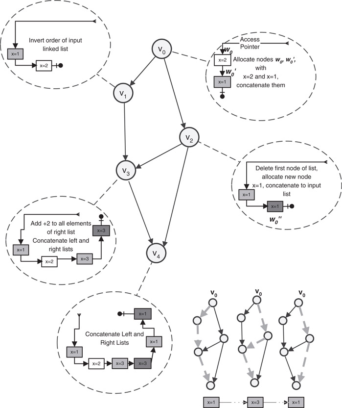
Figure 33.1A DAG of five versions. In each circle we show the corresponding update operation and the resulting version. Nodes with the same color originate from the same seminal node. The three gray nodes in version Dv4 all have the same seminal node (w0′), and are distinguished by their pedigrees 〈v0, v1, v3, v4〉, 〈v0, v2, v3, v4〉, and 〈v0, v2, v4〉.
The basic simulation of Fiat and Kaplan is called the full path method and it works as follows. The data structure consists of a collection of fat nodes. Each fat node corresponds to an explicit allocation of a node by an update operation or in another words, to some seminal node of the naive scheme. For example, the update operations of Figure 33.1 performs 3 allocations (3 seminal nodes) labeled w0, w0′, and w0′′, so our data structure will have 3 fat nodes, f(w0), f(w0′) and f(w0′′). The full path method represents a node w of the naive scheme by a pointer to the fat node representing s(w), together with the pedigree p(w). Thus a single fat node f represents all nodes sharing the same seminal node. We denote this set of nodes by N(f). Note that N(f) may contain nodes that co-exist within the same version and nodes that exist in different versions. A fat node contains the same fields as the corresponding seminal node. Each of these fields, however, rather than storing a single value as in the original node stores a dynamic table of field values in the fat node. The simulation will be able to find the correct value in node w ∈ N(f) using p(w). To specify the representation of a set of values we need the following definition of an assignment pedigree.
Let p ≠ 〈v0,…, vk ≠ u〉 be the pedigree of a node w ∈ Du. Let wk ≠ w, wk − 1,…, w1, wi ∈ Dvi be the sequence of nodes such that wi ∈ Dvi is derived from wi − 1 ∈ Dvi − 1. This sequence exists by the definition of node’s pedigree. Let A be a field in w and let j be the maximum such that there has been an assignment to field A in wj during the update that created vj. We define the assignment pedigree of a field A in node w, denoted by p(A, w), to be the pedigree of wj, that is, p(A, w) ≠ 〈v0, v1,…, vj〉.
In the example of Figure 33.1 the nodes contain one pointer field (named next) and one data field (named x). The assignment pedigree of x in the 1st node of Dv4 is simply 〈v0〉, the assignment pedigree of x in the 2nd node of Dv4 is likewise 〈v0〉, the assignment pedigree of x in the 3rd node of Dv4 is 〈v0, v2, v3〉. Pointer fields also have assignment pedigrees. The assignment pedigree of the pointer field in the 1st node of Dv4 is 〈v0, v1〉, the assignment pedigree of the pointer field in the 2nd node of Dv4 is 〈v0, v1, v3〉, the assignment pedigree of the pointer field of the 3rd node of Dv4 is 〈v0, v2〉, finally, the assignment pedigree of the pointer field of the 4th node of Dv4 is 〈v2, v3, v4〉.
We call the set {p(A, w)|w ∈ N(f)} the set of all assignment pedigrees for field A in a fat note f, and denote it by P(A, f). The table that represents field A in fat node f contains an entry for each assignment pedigree in P(A, f). The value of a table entry, indexed by an assignment pedigree p ≠ 〈v0, v1,…, vj〉, depends on the type of the field as follows. If A is a data field then the value stored is the value assigned to A in the node wj ∈ Dvj whose pedigree is p. If A is a pointer field then let w be the node pointed to by field A after the assignment to A in wj. We store the pedigree of w and the address of the fat node that represents the seminal node of w.
An access pointer to a node w in version v is represented by a pointer to the fat node representing the seminal node of w and the pedigree of w.
In Figure 33.2 we give the fat nodes of the persistent data structure given in Figure 33.1. For example, the field next has three assignments in nodes of N(f(w0′)). Thus, there are three assignment pedigrees in P(next, f(w0′)):
1.〈v0〉—allocation of w0′ in version Dv0 and default assignment of null to next.
2.〈v0, v1〉—inverting the order of the linked list in version Dv1 and thus assigning next a new value. The pointer is to a node whose pedigree is 〈v0, v1〉 and whose seminal node is w0. So we associate the value (〈v0, v1〉, f(w0)) with 〈v0, v1〉.
3.〈v0, v2〉—allocating a new node, w0′′, in version Dv2, and assigning next to point to this new node. The pedigree of w0′′ is 〈v2〉 so we associate the value (〈v2〉, f(w0′′)) with 〈v0, v2〉.
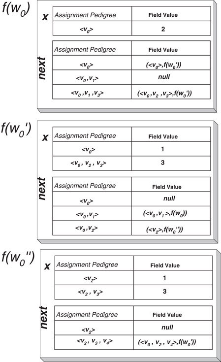
Figure 33.2The fat nodes for the example of Figure 33.1.
You can see all three entries in the table for next in the fat node f(w0′) (Figure 33.2). Similarly, we give the table for field x in f(w0′) as well as the tables for both fields in fat nodes f(w0) and f(w0′′).
When we traverse the data structure we are pointing to some fat node f and hold a pedigree q of some node w whose seminal node corresponds to f and we would like to retrieve the value of field A in node w from the table representing field A in f. We do that as follows. First we identify the assignment pedigree p(A, w) of field A in node w. This is the longest pedigree which is a prefix of q and has an entry in this table. In case A is a data field, the value we are after is simply the value associated with p(A, w). However if A is a pointer field then the value stored with p(A, w) may not be the value of A in w. This value identifies a node in the version where the assignment occurred, whereas we are interested in a node in the version of w that this pointer field points to.
Let q ≠ 〈q0,…, qk〉 and let p(A, w) ≠ 〈q0, q1,…, qj〉. Let the value of p(A, w) be (t, f), where t is the pedigree of the target node in Dqj and f is the fat node representing the seminal node of this target node. The nodes identified by the pedigrees p(A, w) and t were copied in versions qj + 1,…, qk without any assignment made to field A in the nodes derived from the node whose pedigree is p(A, w). Thus the pedigree of the target node of field A of node w in Dqk is t∥〈qj + 1,…, qk〉, where ∥ represents concatenation.
It follows that we need representations for pedigrees and the tables representing field values that support an efficient implementation of the followings.
1.Given a pedigree q find the longest prefix of q stored in a table.
2.Given a pedigree q, replace a prefix of q with another pedigree p.
3.To facilitate updates we also need to be able to add a pedigree to a table representing some field with a corresponding value.
In their simplest simulation Fiat and Kaplan suggested to represent pedigrees as linked lists of version numbers, and to represent tables with field values as tries. Each assignment pedigree contained in the table is represented by a path in the corresponding trie. The last node of the path stores the associated value. Nodes in the trie can have large degrees so for efficiency we represent the children of each node in a trie by a splay tree.
Let U be the total number of assignments the simulation performs and consider the update creating version v. Then with this implementation each assignment performed during this update requires O(d(v)) words of size O(log U) bits, and takes O(d(v) + log U) time, where d(v) is the depth of v in the DAG. Field retrieval also takes O(d(v) + log U) time.
The second method suggested by Fiat and Kaplan is the compressed path method. The essence of the compressed path method is a particular partition of our DAG into disjoint trees. This partition is defined such that every path enters and leaves any specific tree at most once. The compressed path method encodes paths in the DAG as a sequence of pairs of versions. Each such pair contains a version where the path enters a tree T and the version where the path leaves the tree T. The length of each such representation is O(e(D)).* Each value of a field in a fat node is now associated with the compressed representation of the path of the node in N(f) in which the corresponding assignment occurred. A key property of these compressed path representations is that they allow easy implementation of the operations we need to perform on pedigree, like replacing a prefix of a pedigree with another pedigree when traversing a pointer. With the compressed path method each assignment requires up to O(e(D)) words each of bits. Searching or updating the trie representing all values of a field in a fat node requires time. For the case where the DAG is a tree this method degenerates to the fat node simulation of [1].
Fiat and Kaplan also suggested how to use randomization to speed up their two basic methods at the expense of (slightly) larger space expansion and polynomially small error probability. The basic idea is encode each path (or compressed path) in the DAG by an integer. We assign to each version a random integer, and the encoding of a path p is simply the sum of the integers that correspond to the versions on p. Each value of a field in a fat node is now associated with the integer encoding the path of the node in N(f) in which the corresponding assignment occurred. To index the values of each field we use a hash table storing all the integers corresponding to these values.
To deal with values of pointer fields we have to combine this encoding with a representation of paths in the DAG (or compressed paths) as balanced search trees, whose leaves (in left to right order) contain the random integers associated with the vertices along the path (or compressed path). This representation allows us to perform certain operations on these paths in logarithmic (or poly-logarithmic) time whereas the same operations required linear time using the simpler representation of paths in the non-randomized methods.
33.4Making Specific Data Structures More Efficient
The purely functional deques of Kaplan and Tarjan [11], the confluently persistent deques of Kaplan, Okasaki, and Tarjan [14], the purely functional heaps of Brodal and Okasaki [33], and the purely functional finger search trees of Kaplan and Tarjan [19], are all based on a simple and useful mechanism called redundant counters, which to the best of our knowledge first appeared in lecture notes by Clancy and Knuth [15]. In this section we describe what redundant counters are, and demonstrate how they are used in simple persistent deques data structure.
A persistent implementation of deques support the following operations: q′ ≠ push(x, q): Inserts an element x to the beginning of the deque q returning a new deque q′ in which x is the first element followed by the elements of q. (x, q′) ≠ pop(q): Returns a pair where x is the first element of q and q′ is a deque containing all elements of q but x. q′ ≠ Inject(x, q): Inserts an element x to the end of the deque q returning a new deque q′ in which x is the last element preceded by the elements of q. (x, q′) ≠ eject(q): Returns a pair where x is the last element of q and q′ is a deque containing all elements of q but x. A stack supports only push and pop, a queue supports only push and eject. Catenable deques also support the operation q ≠ catenate(q1, q2): Returns a queue q containing all the elements of q1 followed by the elements of q2.
Although queues, and in particular catenable queues, are not trivial to make persistent, stacks are easy. The regular representation of a stack by a singly linked list of nodes, each containing an element, ordered from first to last, is in fact purely functional. To push an element onto a stack, we create a new node containing the new element and a pointer to the node containing the previously first element on the stack. To pop a stack, we retrieve the first element and a pointer to the node containing the previously second element.
Direct ways to make queues persistent simulate queues by stacks. One stack holds elements from the beginning of the queue and the other holds elements from its end. If we are interested in fully persistence this simulation should be real time and its details are not trivial. For a detailed discussion see Kaplan and Tarjan [11] and the references there.
Kaplan and Tarjan [11] described a new way to do a simulation of a deque with stacks. They suggest to represent a deque by a recursive structure that is built from bounded-size deques called buffers. Buffers are of two kinds: prefixes and suffixes. A non-empty deque q over a set A is represented by an ordered triple consisting of a prefix, prefix(q), of elements of A, a child deque, child(q), whose elements are ordered pairs of elements of A, and a suffix, suffix(q), of elements of A. The order of elements within q is the one consistent with the orders of all of its component parts. The child deque child(q), if non-empty, is represented in the same way. Thus the structure is recursive and unwinds linearly. We define the descendants {childi( q)} of deque d in the standard way, namely child0(q) ≠ q and childi + 1(q) ≠ child(childi(q)) for i ≥ 0 if childi(q) is non-empty.
Observe that the elements of q are just elements of A, the elements of child(q) are pairs of elements of A, the elements of child(child(q)) are pairs of pairs of elements of A, and so on. One can think of each element of childi(q) as being a complete binary tree of depth i, with elements of A at its 2i leaves. One can also think of the entire structure representing q as a stack (of q and its descendants), each element of which is prefix-suffix pair. All the elements of q are stored in the prefixes and suffixes at the various levels of this structure, grouped into binary trees of the appropriate depths: level i contains the prefix and suffix of childi(q). See Figure 33.3.
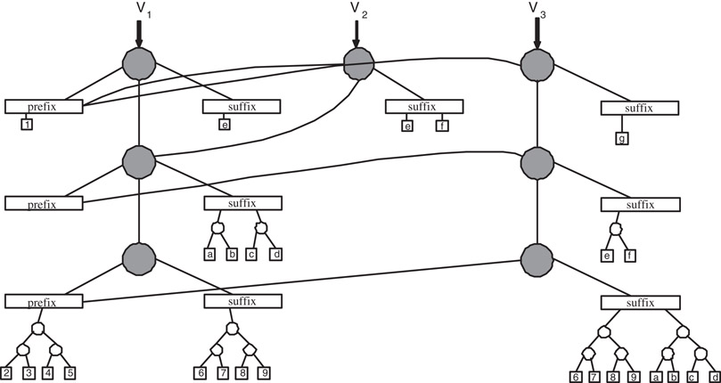
Figure 33.3Representation of a deque of elements over A. Each circle denotes a deque and each rectangle denotes a buffer. Squares correspond to elements from A which we denote by numbers and letters. Each buffer contains 0, 1, or 2 elements. Three versions are shown V1, V2, and V3. Version V2 was obtained from V1 by injecting the element f. Version V3 obtained from version V2 by injecting the element g. The latter inject triggered two recursive injects into the child and grandchild deques of V2. Note that identical binary trees and elements are represented only once but we draw them multiple times to avoid cluttering of the figure.
Because of the pairing, we can bring two elements up to level i by doing one pop or eject at level i + 1. Similarly, we can move two elements down from level i by doing one push or inject at level i + 1. This two-for-one payoff leads to real-time performance.
Assume that each prefix or suffix is allowed to hold 0, 1, or 2 elements, from the beginning or end of the queue, respectively. We can implement q′ ≠ push(x, q) as follows. If the prefix of q contains 0 or 1 elements we allocate a new node to represent q′ make its child deque and its suffix identical to the child and suffix of q, respectively. The prefix of q′ is a newly allocated prefix containing x and the element in the prefix of q, if the prefix of q contained one element. We return a pointer the new node which represents q′. For an example consider version V2 shown in Figure 33.3 that was obtained from version V1 by a case of inject symmetric to the case of the push just described.
The hard case of the push is when the prefix of q already contains two elements. In this case we make a pair containing these two elements and push this pair recursively into child(q). Then we allocate a new node to represent q′, make its suffix identical to the suffix of q, make the deque returned by the recursive push to child(q) the child of q′, and make the prefix of q′ be a newly allocated prefix containing x. For an example consider version V3 shown in Figure 33.3 that was obtained from version V2 by a recursive case of inject symmetric to the recursive case of the push just described. The implementations of pop and eject is symmetric.
This implementation is clearly purely functional and therefore fully persistent. However the time and space bounds per operation are O(log n). The same bounds as one gets by using search trees to represent the deques with the path copying technique. These logarithmic time bounds are by far off from the ephemeral O(1) time and space bounds.
Notice that there is a clear correspondence between this data structure and binary counters. If we think of a buffer with two elements as the digit 1, and of any other buffer as the digit 0, then the implementation of push(q) is similar to adding one to the binary number defined by the prefixes of the queues childi(q). It follows that if we are only interested in partially persistent deques then this implementation has O(1) amortized time bound per operation (see the discussion of binary counters in the next section). To make this simulation efficient in a fully persistent setting and even in the worst case, Kaplan and Tarjan suggested to use redundant counters.
33.4.1Redundant Binary Counters
To simplify the presentation we describe redundant binary counters, but the ideas carry over to any basis. Consider first the regular binary representation of an integer i. To obtain from this representation the representation of i + 1 we first flip the rightmost digit. If we flipped a 1 to 0 then we repeat the process on the next digit to the left. Obviously, this process can be long for some integers. But it is straightforward to show that if we carry out a sequence of such increments starting from zero then on average only a constant number of digits change per increment.* Redundant binary representations (or counters as we will call them) address the problem of how to represent i so we can obtain a representation of i + 1 while changing only a constant number of digits in the worst case.
A redundant binary representation, d, of a non-negative integer x is a sequence of digits dn,…, d0, with di ∈ {0,1,…,2}, such that . We call d regular if, between any two digits equal to 2, there is a 0, and there is a 0 between the rightmost 2 and the least significant digit. Notice that the traditional binary representation of each integer (which does not use the digit 2) is regular. In the sequel when we refer to a regular representation we mean a regular redundant binary representation, unless we explicitly state otherwise.
Suppose we have a regular representation of i. We can obtain a regular representation of i + 1 as follows. First we increment the rightmost digit. Note that since the representation of i is regular, its rightmost digit is either 0 or 1. So after the increment the rightmost digit is either 1 or 2 and we still have a redundant binary representation for i + 1. Our concern is that this representation of i + 1 may not be regular. However, since the representation of i we started out with was regular the only violation to regularity that we may have in the representation of i + 1 is lacking a 0 between the rightmost 2 and the least significant digit. It is easy to check that between any two digits equal to 2, there still is a 0, by the regularity of i.
We can change the representation of i + 1 to a representation which is guaranteed to be regular by a simple fix operation. A fix operation on a digit di ≠ 2 increments di + 1 by 1 and sets di to 0, producing a new regular representation d′ representing the same number as d.* If after incrementing the rightmost digit we perform a fix on the rightmost 2 then we switch to another representation of i + 1 that must be regular. We omit the proof here which is straightforward.
It is clear that the increment together with the fix that may follow change at most three digits. Therefore redundant binary representations allow to perform an increment while changing constantly many digits. However notice that in any application of this numbering system we will also need a representation that allows to get to the digits which we need to fix efficiently. We show one such representation in the next section.
These redundant representations can be extended so we can also decrement it while changing only a constant number of digits, or even more generally so that we can increment or decrement any digit (add or subtract 2i) while changing a constant number of other digits. These additional properties of the counters were exploited by other applications (see, e.g., [19,34]).
Kaplan and Tarjan use this redundant binary system to improve the deque implementation we described above as follows. We allow each of the prefixes and suffixes to contain between 0 and 5 elements. We label each buffer, and each deque, by one of the digits 0, 1, and 2. We label a buffer 0 if it has two or three elements, we label it 1 if it has one or four elements, and we label it 2 if it has zero or five elements. Observe that we can add one element to or delete one element from a buffer labeled 0 or 1 without violating its size constraint: A buffer labeled 0 may change its label to 1, and a buffer labeled 1 may change its label to 2. (In fact a 1 can also be changed to 0 but this may not violate regularity.) The label of a deque is the larger among the labels of its buffers, unless its child and one of its buffers are empty, in which case the label of the deque is identical to the label of its nonempty buffer.
This coloring of the deques maps each deque to a redundant binary representation. The least significant digit of this representation is the digit of q, the next significant digit is the digit of child(q), and, in general, the ith significant digit is the digit corresponding to childi(q) if the latter is not empty. We impose an additional constraint on the deques and require that the redundant binary representation of any top-level deque is regular.
A regular top-level deque is labeled 0 or 1 which implies that both its prefix and its suffix are labeled 0 or 1. This means that any deque operation can be performed by operating on the appropriate top-level buffer. Suppose that the operation is either a push or a pop, the case of inject and eject is symmetric. We can construct the resulting queue q′ by setting child(q′) ≠ child(q) and suffix(q′) ≠ suffix(q). The prefix of q′ is a newly allocated buffer that contains the elements in prefix(q) together with the new element in case of push or without the first element in case of pop. Clearly all these manipulations take constant time.
The label of q′, however, may be one larger than the label of q. So the redundant binary representation corresponding to q′ is either the same as the redundant binary representation of q in which case it is regular, or it is obtained from the redundant binary representation of q by incrementing the least significant digit. (The least significant digit can also decrease in which case regularity is also preserved.) This corresponds to the first step in the increment procedure for redundant regular representations described in the previous section.
To make the redundant binary representation of q′ regular we may have to apply a fix operation. Let i be the minimum such that childi(q′) is labeled 2. If for all j < i, childj(q′) is labeled 1 then the fix has to change the label of childi(q′) to 0 and increment the label of childi + 1(q′).
Fortunately, we have an appropriate interpretation for such a fix. Assume childi + 1(q′) have a non-empty child. (We omit the discussion of the case where childi + 1(q′) have an empty child which is similar.) We know that the label of childi + 1(q′) is either 0 or 1 so neither of its buffers is empty or full. If the prefix of childi(q′) has at least four elements we eject 2 of these elements and push them as a single pair to the prefix of childi + 1(q′). If the prefix of childi(q′) has at most one element we pop a pair from the prefix of childi + 1(q′) and inject the components of the pair into the prefix of childi(q′). This makes the prefix of childi(q′) containing either two or three elements. Similarly by popping a pair from or pushing a pair to the suffix of childi(q′), and injecting a pair to or ejecting a pair from the suffix of childi + 1(q′) we make the suffix of childi(q′) containing two or three elements. As a result the label of childi(q′) and its two buffers becomes 0 while possibly increasing the label of one or both buffers of childi + 1(q′) and thereby the label of childi + 1(q′) as well.
There is one missing piece for this simulation to work efficiently. The topmost deque labeled 2 may be arbitrarily deep in the recursive structure of q′, since it can be separated from the top level by many deques labeled 1. To implement the fix efficiently we have to be able to find this deque fast and change it in a purely functional way by copying the deques that change without having to copy all their ancestors deques.
For this reason we do not represent a deque in the obvious way, as a stack of prefix-suffix pairs. Instead, we break this stack up into substacks. There is one substack for the top-level deque and one for each descendant deque labeled 0 or 2 not at the top level. Each substack consists of a top-level, or a deque labeled 0, or a deque labeled 2 and all consecutive proper descendant deques labeled 1. We represent the entire deque by a stack of substacks of prefix-suffix pairs using this partition into substacks. This can be realized with four pointers per each node representing a deque at some level. Two of the pointers are to the prefix and suffix of the deque. One pointer is to the node for the child deque if this deque is non-empty and labeled 1. One pointer is to the node of the nearest proper descendant deque not labeled 1, if such a deque exists and q itself is not labeled 1 or top-level. See Figure 4.2.
A single deque operation will require access to at most the top three substacks, and to at most the top two elements in any such substack. The label changes caused by a deque operation produce only minor changes to the stack partition into substacks, changes that can be made in constant time. In particular, changing the label of the top-level deque does not affect the partition into substacks. Changing the label of the topmost deque which is labeled 2 to 0 and the label of its child from 1 to 2 splits one substack into its first element, now a new substack, and the rest. This is just a substack pop operation. Changing the label of the topmost deque which is labeled 2 to 0 and the label of its child from 0 to 1 merges a singleton substack with the substack under it. This is just a substack push operation.
To add catenation, Kaplan and Tarjan had to change the definition of the data structure and allow deques to be stored as components of elements of recursive deques. The redundant binary numbering system, however, still plays a key role. To represent a catenable deque, Kaplan and Tarjan use noncatenable deques as the basic building blocks. They define a triple over a set A recursively as a prefix of elements of A, a possibly empty deque of triples over A, and a suffix of elements of A, where each prefix or suffix is a noncatenable deque. Then, they represent a catenable deque of elements from A by either one or two triples over A. The underlying skeleton of this structure is a binary tree (or two binary trees) of triples. The redundant binary number system is extended so that it can distribute work along these trees by adding an extra digit.
Kaplan, Okasaki, and Tarjan [14] simplified these data structures at the expense of making the time bounds amortized rather than worst case and using assignment, thus obtaining a confluently persistent data structure which is not purely functional. The key idea underlying their data structure is to relax the rigid constraint of maintaining regularity. Instead, we “improve” the representation of a deque q with full or empty prefix when we try to push or pop an element from it. Similarly, with full or empty suffix. This improvement in the representation of q is visible to all deques that contain q as a subdeque at some level and prevents from pushing into deques with full prefixes or popping from deques with empty prefixes from happening too often.
More specifically, assume that we push into a deque q with full prefix. First, we eject two elements from this prefix, make a pair containing them, and push the pair recursively into child(q). Let the result of the recursive push be child′(q). Then we change the representation of q so that it has a new prefix which contains all the elements in the prefix of q but the two which we ejected, and its child deque is child′(q). The suffix of q does not change. Finally we perform the push into q by creating a new queue q′ that has the same suffix and child deque as q, but has a new prefix that contains the elements in the prefix of q together with the new element. A careful but simple analysis shows that each operation in this implementation takes O(1) amortized time. By extending this idea, Kaplan, Okasaki, and Tarjan managed to construct catenable deques using only constant size buffers as the basic building blocks.
33.5Concluding Remarks and Open Questions
Much progress has been made on persistent data structures since the seminal paper of Driscoll et al. [1]. This progress has three folds: In developing general techniques to make any data structure persistent, in making specific data structures persistent, and in emerging algorithmic applications. Techniques developed to address these challenges sometimes proved useful for other applications as well.
This algorithmic field still comprise intriguing challenges. In developing general techniques to make data structures persistent, a notable challenge is to find a way to make the time slowdown of the node splitting method worst case. Another interesting research track is how to restrict the operations that combine versions in a confluently persistent setting so that better time bounds, or simpler simulations, are possible. We also believe that the techniques and data structures developed in this field would prove useful for numerous forthcoming applications.
This work was supported, in part, by the Israel Science Foundation (ISF) under grant 548/00.
1.J. R. Driscoll, N. Sarnak, D. Sleator, and R. Tarjan. Making data structures persistent. J. of Computer and System Science, 38:86–124, 1989.
2.P. F. Dietz and R. Raman. Persistence, amortization and randomization. In Proc. 2nd annual ACM-SIAM symposium on Discrete algorithms, pages 78–88. Society for Industrial and Applied Mathematics, 1991.
3.G. S. Brodal. Partially persistent data structures of bounded degree with constant update time. Nordic J. of Computing, 3(3):238–255, 1996.
4.P. F. Dietz. Fully persistent arrays. In Proc. 1st Worksh. Algorithms and Data Structures (WADS 1989), volume 382 of Lecture Notes in Computer Science, pages 67–74. Springer, 1989.
5.P. van Emde Boaz, R. Kaas, and E. Zijlstra. Design and implementation of an efficient priority queue. Mathematical Systems Theory, 10:99–127, 1977.
6.P. van Emde Boaz. Preserving order in a forest in less than logarithmic time. Information Processing Letters, 6(3):80–82, 1977.
7.A. Fiat and H. Kaplan. Making data structures confluently persistent. J. of Algorithms, 48(1):16–58, 2003. Symposium on Discrete Algorithms.
8.D. P. Dobkin and J. I. Munro. Efficient uses of the past. J. of Algorithms, 6:455–465, 1985.
9.M. H. Overmars. Searching in the past, I. Technical Report RUU-CS-81-7, Department of Computer Science, University of Utrecht, Utrecht, The Netherlands, 1981.
10.B. Chazelle. How to search in history. Information and Control, 64:77–99, 1985.
11.H. Kaplan and R. E. Tarjan. Purely functional, real-time deques with catenation. J. of the ACM, 46(5):577–603, 1999.
12.J. Driscoll, D. Sleator, and R. Tarjan. Fully persistent lists with catenation. J. of the ACM, 41(5):943–959, 1994.
13.A. L. Buchsbaum and R. E. Tarjan. Confluently persistent deques via data structural bootstrapping. J. of Algorithms, 18:513–547, 1995.
14.H. Kaplan, C. Okasaki, and R. E. Tarjan. Simple confluently persistent catenable lists. Siam J. on Computing, 30(3):965–977, 2000.
15.M. J. Clancy and D. E. Knuth. A programming and problem-solving seminar. Technical Report STAN-CS-77-606, Department of Computer Science, Stanford University, Palo Alto, 1977.
16.C. Okasaki. Amortization, lazy evaluation, and persistence: Lists with catenation via lazy linking. In IEEE Symposium on Foundations of Computer Science, pages 646–654, 1995.
17.R. E. Tarjan and J. Van Leeuwen. Worst case analysis of set union algorithms. J. of the ACM, 31:245–281, 1984.
18.R. E. Tarjan. Data Structures and Network algorithms. SIAM, Philadelphia, 1982.
19.H. Kaplan and R. E. Tarjan. Purely functional representations of catenable sorted lists. In Proc. 28th Annual ACM Symposium on Theory of Computing, pages 202–211. ACM Press, 1996.
20.N. Sarnak and R. E. Tarjan. Planar point location using persistent search trees. Communications of the ACM, 29(7):669–679, 1986.
21.D. P. Dobkin and R. J. Lipton. Multidimensional searching problems. SIAM J. on Computing, 5(2):181–186, 1976.
22.R. Cole. Searching and storing similar lists. J. of Algorithms, 7:202–220, 1986.
23.A. Boroujerdi and B. Moret. Persistence in computational geometry. In Proc. 7th Canadian Conf. Comp. Geometry (CCCG 95), pages 241–246, 1995.
24.E. M. McCreight. Priority search trees. Siam J. on Computing, 14:257–276, 1985.
25.S. Alstrup, G. S. Brodal, I. L. Gørtz, and T. Rauhe. Time and space efficient multi-method dispatching. In Proc. 8th Scandinavian Workshop on Algorithm Theory, volume 2368 of Lecture Notes in Computer Science, pages 20–29. Springer, 2002.
26.N. Kitsios and A. Tsakalidis. Space reduction and an extension for a hidden line elimination algorithm. Computational Geometry, 6(6):397–404, 1996.
27.O. Nurmi. A fast line sweep algorithm for hidden line elimination. BIT, 25(3):466–472, 1985.
28.P. Bozanis, N. Kitsios, C. Makris, and A. Tsakalidis. The space-optimal version of a known rectangle enclosure reporting algorithm. Information Processing Letters, 61(1):37–41, 1997.
29.P. Gupta, R. Janardan, H. M. Smid, and B. DasGupta. The rectangle enclosure and point-dominance problems revisited. International J. of Computational Geometry and Applications, 7(5):437–455, 1997.
30.P. F. Dietz and D. D. Sleator. Two algorithms for maintaining order in a list. In Proc. 19th Annual ACM Symposium on Theory of Computing, pages 365–372, 1987.
31.M. A. Bender, R. Cole, E. D. Demaine, M. Farach-Colton, and J. Zito. Two simplified algorithms for maintaining order in a list. In Proc. 10th Annual European Symposium on Algorithms (ESA 2002), volume 2461 of Lecture Notes in Computer Science, pages 152–164. Springer, 2002.
32.M. Dietzfelbinger, A. Karlin, K. Mehlhorn, M. Meyer auf der Heide, H. Rohnert, and R. E. Tarjan. Dynamic perfect hashing: Upper and lower bounds. SIAM J. on Computing, 23(4):738–761, 1994.
33.G. S. Brodal and C. Okasaki. Optimal purely functional priority queues. J. of Functional Programming, 6(6):839–858, 1996.
34.H. Kaplan, N. Shafrir, and R. E. Tarjan. Meldable heaps and boolean union-find. In Proc. 34th Annual ACM Symposium on Theory of Computing (STOC), pages 573–582, 2002.
*This chapter has been reprinted from first edition of this Handbook, without any content updates.
*Note that testing whether a point is above or below a line takes O(1) time.
*We can compress the sparse arrays using hashing but even if we do that the space requirement may be quadratic in m.
*If the update operation that created version i assigned to a particular field more than once we keep only the value that was assigned last.
*We assume that each field has only one value in any particular version. When we update a field in version i that already has a value stamped with version i then we overwrite its previous value.
*So we cannot simply overwrite a value in a predecessor pointer.
*Recall that e(D) is the logarithm of the maximum number of different paths from the root of the DAG to any particular version.
*The rightmost digit changes every increment, the digit to it left changes every other operation, and so on.
*We use the fix only when we know that di + 1 is either 0 or 1.