38. Succinct Representation of Data Structures

Although computer memories, at all levels of the hierarchy, have grown dramatically over the past few years, increased problem sizes continues to outstrip this growth. Minimizing space is crucial not only in keeping data in the fastest memory possible, but also in moving it from one level to another, be it from main memory to cache or from a web site around the world. Standard data compression, say Huffman code or grammar based code, applied to a large text file reduces space dramatically, but basic operations on the text require that it be fully decoded.

In this chapter we focus on representations that are not only terse but also permit the basic operations one would expect on the underlying data type to be performed quickly. Jacobson [1] seems to have been the first to apply the term succinct to such structures; the goal is to use the information-theoretic minimum number of bits and to support the expected operations on the data type in optimal time. Our archetypical example (discussed in Section 38.4) is the representation of a binary tree. Suppose, we would like to support the operations of navigating through a binary tree moving to either child or the parent of the current node, asking the size of the subtree rooted at the current node or giving the unique “number” of the node so that data can be stored in that position of an array. At $\lg n$ $\lg n$ bits per reference, this adds up to at least $5 n \lg n$ $5 n \lg n$ bits. However, there are only $(\begin{matrix} 2 n + 1 \\ n \end{matrix}) / (2 n + 1)$ $(\begin{matrix} 2 n + 1 \\ n \end{matrix}) / (2 n + 1)$ binary trees, so the information-theoretic minimum space is fewer than 2n bits. Our archetypical data structure is a 2n + o(n)-bit representation that supports the operations noted above, and others, in constant time.

We consider a variety of abstract data types, or combinatorial objects, with the goal of producing such succinct data structures. Most, though not all, of the structures we consider are static. In most cases the construction of a succinct data structure from the standard representation is fairly straightforward in linear time.

Memory Model: We study the problems under the RAM model with word size $Θ (\lg n)$ $Θ (\lg n)$ , where n is the input size of the problem under consideration. This supports arithmetic (addition, subtraction, multiplication and division), indexing and bit-wise boolean operations (AND, OR, NOT, XOR etc.) on words, and reading/writing of words from/to the memory in constant time.

38.2Bitvector

A bitvector provides a simple way to represent a set from any universe that is easily mapped onto [m].^* Membership queries (checking whether a given element from the universe is present in the set) can be answered in constant time (in fact a single bit probe) using a bitvector. Furthermore, one can easily support updates (inserting and deleting elements) in constant time. The most interesting twist on the bitvector came with Jacobson [1] considering two more operations:

•rank(i): return the number of 1s before the position i, and

•select(i): return the position of the ith 1.

As we shall see, these operations are crucial to a number of more complex structures supporting a variety of data types. An immediate use is to support the queries:

•predecessor(x): find the largest element y ≤ x in the set S,

•successor(x): find the smallest element y ≥ x in the set S.

Given a bitvector of length m, Jacobson [1] gave a structure that takes o(m) bits of additional space and supports rank and select operations by making $O (\lg m)$ $O (\lg m)$ bit probes to the structure. On a RAM with word size $Θ (\lg m)$ $Θ (\lg m)$ bits, the structure given by Munro [2] enhanced this structure and the algorithms to support the operations in O(1) time, without increasing the space bound. We briefly describe the details of this structure (Figure 38.1).

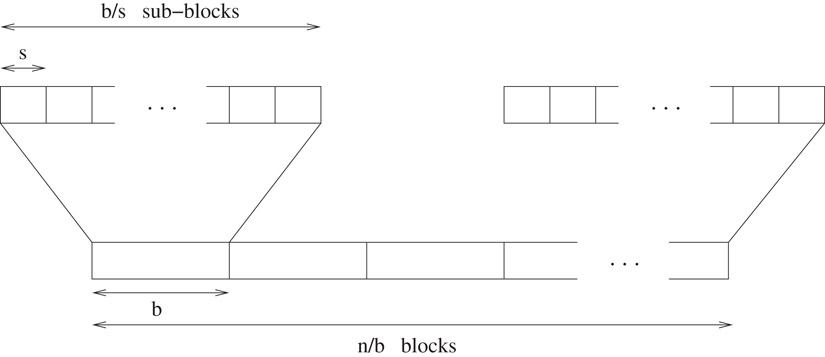
Figure 38.1Two-level rank directory.

The structure for computing rank, the rank directory, consists of the following:

•Conceptually break the bitvector into blocks of length $⌈ \lg^{2} m ⌉$ $⌈ \lg^{2} m ⌉$ . Keep a table containing the number of 1s up to the last position in each block. This takes $O (m / \lg m)$ $O (m / \lg m)$ bits of space.

•Conceptually break each block into sub-blocks of length $⌈ (1 / 2) \lg m ⌉$ $⌈ (1 / 2) \lg m ⌉$ . Keep a table containing the number of 1s within the block up to the last position in each sub-block. This takes $O (m \lg \lg m / \lg m)$ $O (m \lg \lg m / \lg m)$ bits.

•Keep a precomputed table giving the number of 1s up to every possible position in every possible distinct sub-block. Since there $O (\sqrt{m})$ $O (\sqrt{m})$ distinct possible blocks, and $O (\lg m)$ $O (\lg m)$ positions in each, this takes $O (\sqrt{m} \lg m \lg \lg m)$ $O (\sqrt{m} \lg m \lg \lg m)$ bits.

Thus, the total space occupied by this auxiliary structure is o(m) bits. The rank of an element is, then, simply the sum of three values, one from each table.

The structure for computing select uses three levels of directories and is more complex. The first one records the position of every $(\lg m \lg \lg m)$ $(\lg m \lg \lg m)$ th 1 bit in the bitvector. This takes $O (m / \lg \lg m)$ $O (m / \lg \lg m)$ bits. Let r be the subrange between two values in the first directory, and consider the sub-directory for this range. If $r \geq (\lg m \lg \lg m)^{2}$ $r \geq (\lg m \lg \lg m)^{2}$ then explicitly store the positions of all ones, which requires $O (r / \lg \lg m)$ $O (r / \lg \lg m)$ bits. Otherwise, subdivide the range and store the position (relative to the beginning of this range) of every $(\lg r \lg \lg m)$ $(\lg r \lg \lg m)$ th one bit in the second level directory. This takes $O (r / \lg \lg m)$ $O (r / \lg \lg m)$ bits for each range of size r, and hence $O (m / \lg \lg m)$ $O (m / \lg \lg m)$ bits over the entire bitvector. After one more level of similar range subdivision, the range size will reduce to at most $(\lg \lg m)^{4}$ $(\lg \lg m)^{4}$ . Computing select on these small ranges is performed using a precomputed table. The total space occupied by this auxiliary structure is o(m) bits. The query algorithm is straightforward. See [3,4] for details.

This “indexable bitvector” is used as a substructure in several succinct data structures. To represent a bitvector of length m, it takes m + o(m) bits of space. In general, if nothing is known about the bitvector then any representation needs at least m bits to distinguish between all possible bitvectors, and hence this is close to the optimal space. But if we also know the density (the number of ones) of the bitvector, then the space bound is no longer optimal, in general. The “fully indexable dictionary” described in Section 38.3.2 gives a solution that takes nearly optimal space.

Using the ideas involved in constructing rank and select directories, one can also support the following generalizations of these two operations, using o(m) bits of extra space: Given a bitvector of length m, and a fixed binary pattern p of length up to $(1 - ϵ) \lg m$ $(1 - ϵ) \lg m$ , for some fixed constant 0 < ε < 1

•rank_p(i): return the number of (possibly overlapping) occurrences of p before the position i, and

•select_p(i): return the ith occurrence of the pattern p.

One can extend the ideas of rank and select directories to support indexing into a fixed or variable length encoded text (e.g., Huffman coding, prefix-free encoding etc.) in constant time, using negligible extra space. See [1,4] for some examples.

38.3Succinct Dictionaries

The (static) dictionary problem is to store a subset S of size n so that membership queries can be answered efficiently. In our case, the universe is taken to be the set [m]. This problem has been widely studied and various solutions have been proposed to support membership queries in constant time.

As we have seen in the last section, a bitvector is a simple way of representing a set from a given universe. But this requires m bits of space. Since there are $(\binom{m}{n})$ $(\binom{m}{n})$ sets of size n from a universe of size m, one would require only $B \equiv \lg (\binom{m}{n})$ $B \equiv \lg (\binom{m}{n})$ ( $\approx n (\lg m - \lg n + \lg e)$ $\approx n (\lg m - \lg n + \lg e)$ , when n = o(m)) bits to store a canonical representation of any such set. Thus a bitvector is quite wasteful of space when the set is sparse. A sorted array is another simple representation, but it requires $Θ (\lg n)$ $Θ (\lg n)$ time to answer queries. A fusion tree (see Chapter 40) also takes linear space and supports membership queries in $Θ (\lg n / \lg \lg n)$ $Θ (\lg n / \lg \lg n)$ time. In this section, we consider representations of sets whose space complexity is close to the information theoretic minimum and support queries in constant time. (As all the structures outlined below support membership queries in worst case constant time, we do not mention the query complexity explicitly.)

Fredman, Komlós and Szemerédi [5] gave the first linear space structure for the static dictionary problem. This takes $n \lg m + O (n \sqrt{\lg n} + \lg \lg m)$ $n \lg m + O (n \sqrt{\lg n} + \lg \lg m)$ bits of space. The lower order term was later improved by Schmidt and Siegel [6] to $O (n + \lg \lg m)$ $O (n + \lg \lg m)$ . This structure uses a universe reduction function followed by a two-level hash function to hash the given subset one-to-one onto the set [n], and stores the elements of subset in a hash table (in the order determined by the hash function). The hash table takes $n \lg m$ $n \lg m$ bits and a clever encoding of the hash function takes $O (n + \lg \lg m)$ $O (n + \lg \lg m)$ bits of space. We refer to this as the FKS hashing scheme. Note that the space required for this structure is $Θ (n \lg n)$ $Θ (n \lg n)$ bits more than the optimal bound of $B$ $B$ bits.

Brodnik and Munro [7] gave a static dictionary representation that takes $B + o (B)$ $B + o (B)$ bits of space. It uses two different solutions depending on the relative values of n and m. When the set is relatively sparse (namely, when $n \leq m / (\lg m)^{\lg \lg m}$ $n \leq m / (\lg m)^{\lg \lg m}$ ), it partitions the elements into buckets based on the first $\lg n - \lg \lg m$ $\lg n - \lg \lg m$ bits of their bit representations, and store explicit pointers to refer to the representations of individual buckets. Each bucket is represented by storing all the elements that fall into it in a perfect hash table for that bucket. Otherwise, when the set is dense, it uses two levels of bucketing (at each level splitting the universe into a number of equal-range buckets, depending only on the universe size) after which the range of these buckets reduces to $Θ (\lg n)$ $Θ (\lg n)$ . These small buckets are stored (almost) optimally by storing pointers into a precomputed table that contains all possible small buckets. In either case the space occupancy can be shown to be $B + o (B)$ $B + o (B)$ bits.

Pagh [8] observed that each bucket of the hash table may be resolved with respect to the part of the universe hashing to that bucket. Thus, one can save space by compressing the hash table, storing only the quotient information, rather than the element itself. From the FKS hash function, one can obtain a quotienting function that takes $\lg (m / n) + O (1)$ $\lg (m / n) + O (1)$ bits for each element. Using this idea one can obtain a dictionary structure that takes $n \lg (m / n) + O (n + \lg \lg m)$ $n \lg (m / n) + O (n + \lg \lg m)$ bits of space, which is only Θ(n) bits more than the information-theoretic lower bound (except for the $O (\lg \lg m)$ $O (\lg \lg m)$ term). Pagh has also given a dictionary structure that takes only $B + o (n) + O (\lg \lg m)$ $B + o (n) + O (\lg \lg m)$ bits of space.

38.3.1Indexable Dictionary

One useful feature of the sorted array representation of a set is that, given an index i, the ith smallest element in the set can be retrieved in constant time. Furthermore, when we locate an element in the array, we immediately know its rank (the number of elements in the set which are less than the given element). On the other hand, hashing based schemes support membership in constant time, but typically do not maintain the ordering information. In this section we look at a structure that combines the good features of both these approaches.

An indexable dictionary is a structure representing a set S of size n from the universe [m] to support the following queries in constant time:

•rank(x, S): Given x ∈ [m], return −1 if x ∉ S, and |{y ∈ S|y < x}| otherwise, and

•select(i, S): Given i ∈ {1,…n}, return the ith smallest element in S.

Here the rank operation is only supported for the elements present in the set S. Ajtai [9] showed that the more general problem of supporting rank for every element in the universe has a query lower bound of $Ω (\lg \lg n)$ $Ω (\lg \lg n)$ , even if the space used is polynomial in n. As a consequence, we emphasize the need for handling both S and its complement in the next section.

A dictionary that supports rank operation [10], as well as an indexable dictionary is very useful in representing trees [11] (see Section 38.4.3).

Elias [12] considered the indexable dictionary problem and gave a representation that takes $n \lg m - n \lg n + O (n)$ $n \lg m - n \lg n + O (n)$ bits and supports the queries in O(1) time, though he only considered the average case time complexity of the queries. Raman et al. [11] have given an indexable dictionary structure that takes $B + o (n) + O (\lg \lg m)$ $B + o (n) + O (\lg \lg m)$ bits. The main idea here is, again, to partition the elements into buckets based on their most significant bits, as in the static dictionary structure of Brodnik and Munro [7]. The difference is that instead of storing explicit pointers to the bucket representations, they store the bucket sizes using a succinct representation that supports partial sum queries (see Section 38.8) in constant time. This not only saves a significant amount of space, but also provides the extra functionality needed for supporting rank and select.

Using similar ideas, one can also represent multisets and collections of sets using almost optimal space. See [11] for details.

38.3.2Fully Indexable Dictionary

Given a set S ⊆ [m], a fully indexable dictionary (FID) of S is a representation that supports rank and select operations on both S and its complement $\bar{S} = [m] S$ $\bar{S} = [m] S$ in constant time [11].

It is easy to see that the bitvector representation of a set, with auxiliary structures to support rank and select on both the bits as mentioned in Section 38.2, is an FID. But this requires m + o(m) bits, where m is the size of the universe. Here we look at an FID representation that takes $B + o (m)$ $B + o (m)$ bits of space. Note that when the set is reasonably sparse (namely when $n = m / ω (\lg m)$ $n = m / ω (\lg m)$ ) $B = o (m)$ $B = o (m)$ , and hence it improves the space complexity of the bitvector representation.

Let S ⊆ [m] be a given set of size n. Divide [m] into blocks of consecutive elements, with block size $u = ⌊ \frac{1}{2} \lg m ⌋$ $u = ⌊ \frac{1}{2} \lg m ⌋$ . Let S_i be the subset of S that falls into the ith block. Each of the S_i’s is represented by storing an index into a table that contains the characteristic bitvectors of all possible subsets of a particular size from the universe [u]. As a consequence, the space occupied by these representations together with all the precomputed tables can be shown to be $B + o (m)$ $B + o (m)$ bits. To enable fast access to the representations of these subsets, we store the partial sums of the sizes of the subsets, and also the partial sums of the lengths of the representations of these subsets, which take $O (m \lg \lg m / \lg m)$ $O (m \lg \lg m / \lg m)$ bits. This can be used to support rank in O(1) time.

To support select, we first store the positions of every $(\lg^{2} m)$ $(\lg^{2} m)$ th element explicitly in an array, which takes $O (m / \lg m)$ $O (m / \lg m)$ bits. Call the part the universe that lies between two successive elements in this array a segment. If the size of a segment is more than $\lg^{4} m$ $\lg^{4} m$ , then we explicitly store all the $\lg^{2} m$ $\lg^{2} m$ elements of S that belong to this segment in sorted order. This takes $\lg^{3} m$ $\lg^{3} m$ bits for every such “sparse” segment, and hence at most $m / \lg m$ $m / \lg m$ bits, over all the sparse segments. Dense segments are handled by constructing a complete tree with branching factor $\sqrt{\lg m}$ $\sqrt{\lg m}$ , and so constant height, whose leaves are the blocks that constitute this segment, and storing some additional information to navigate this tree efficiently (see the searchable partial sum structure in Section 38.8).

To support rank and select on $\bar{S}$ $\bar{S}$ , first observe that an implicit representation of a set over a given universe is also an implicit representation of its complement. Thus, we need not store the implicit representations of ${\bar{S}}_{i}$ ${\bar{S}}_{i}$ again. Except for this, we repeat the above construction with S_i’s replaced by ${\bar{S}}_{i}$ ${\bar{S}}_{i}$ ’s.

The overall space requirement of the structure is $B + O (m \lg \lg m / \lg m)$ $B + O (m \lg \lg m / \lg m)$ bits, and rank and select are supported on both S and $\bar{S}$ $\bar{S}$ in O(1) time. See [11] for details.

38.3.3Dynamic Dictionary

We have looked at several succinct structures for static dictionaries. We now briefly consider the dynamic dictionary problem where one can add and delete elements from the set while supporting the membership queries.

Model: The model of memory allocation is very important in dynamic data structures. One widely used model [11,13,14] is to assume the existence of a “system” memory manager that would allocate and free memory in variable-sized chunks. In this model, the space complexity of a structure is counted as the total size of all the blocks allocated for that structure, and hence this approach does not account for the space wastage due to external fragmentation.

Fundamentally, memory is most easily viewed as a large array. If we are to use the storage, we must manage it. Therefore a simple view is to count all the fragmentation we may cause and count the memory usage as the difference between the addresses of the first and last locations used by the structure. While more complex scenarios may be more realistic in certain cases, we take this simple address difference model as our focus. The methods we discuss are equivalent under either model up to constant factors.

A balanced tree can be used to support all the dynamic dictionary operations in $O (\lg n)$ $O (\lg n)$ time using $n \lg m + O (n \lg n)$ $n \lg m + O (n \lg n)$ bits, where n is the current size of the set. Using the ideas of the FKS dictionary, Dietzfelbinger et al. [15] gave a dynamic dictionary structure that supports membership in O(1) time and updates (insert/delete) in O(1) expected amortized time. This structure takes $O (n \lg m)$ $O (n \lg m)$ bits of space. There have been several improvements, lowering the space complexity close to the information theoretic-minimum, culminating in a structure that takes $B + o (B)$ $B + o (B)$ bits with the same query complexity as above. See [7,8,16–18] and the references therein.

All these structures also support associating satellite information with the elements, so that whenever an element is found to be in the set, we can also retrieve the satellite information associated with it in constant time.

38.4Tree Representations

Trees are one of the most fundamental objects in computer science. We consider the problem of representing large trees succinctly. Storing a tree with a pointer per child as well as other structural information can account for the dominant storage cost. For example, standard representations of a binary tree on n nodes, using pointers, take $O (n \lg n)$ $O (n \lg n)$ bits of space. Since there are only $(\begin{matrix} 2 n + 1 \\ n \end{matrix}) / (2 n + 1)$ $(\begin{matrix} 2 n + 1 \\ n \end{matrix}) / (2 n + 1)$ different binary trees on n nodes, less than 2n bits suffice to distinguish between them. We look at some binary tree representations that take 2n + o(n) bits and support the basic navigational operations in constant time.

38.4.1Binary Trees

First, if the tree is a complete binary tree (i.e., a binary tree in which every level, except possibly the deepest, is completely filled, and the last level is filled from the left as far as required), then there is a unique tree of a given size and we require no additional space to store the tree structure. In fact, by numbering the nodes from 1 to n in the “heap order” [19] (left-to-right level-order traversal of the tree), one can support navigational operations on the tree by observing that the parent of a node numbered i is the node numbered $⌊ i / 2 ⌋$ $⌊ i / 2 ⌋$ , and the left and right children of node i are 2i and 2i + 1 respectively. But this property does not hold when the tree is not complete.

If the tree is not complete, one could extend it to a complete binary tree with the same height and store a bit vector indicating which nodes are present in the tree (in the heap order of the complete tree) to support the operations efficiently. But this takes space exponential in the number of nodes, in the worst case.

To save space, one can use the following compressed representation due to Jacobson [1]: First, mark all the nodes of the tree with 1 bits. Then add external nodes to the tree, and mark them with 0 bits. Construct a bitvector by reading off the bits that are marking the nodes in left-to-right level-order. (See Figure 38.2.) It is easy to see that the original tree can be reconstructed from this bitvector. For a binary tree with n nodes, this bitvector representation takes 2n + 1 bits. Moving between parent and child is just a slight twist on the method used in a heap. By storing the rank and select directories for this bitvector, one can support the navigational operations in constant time using the following equations:

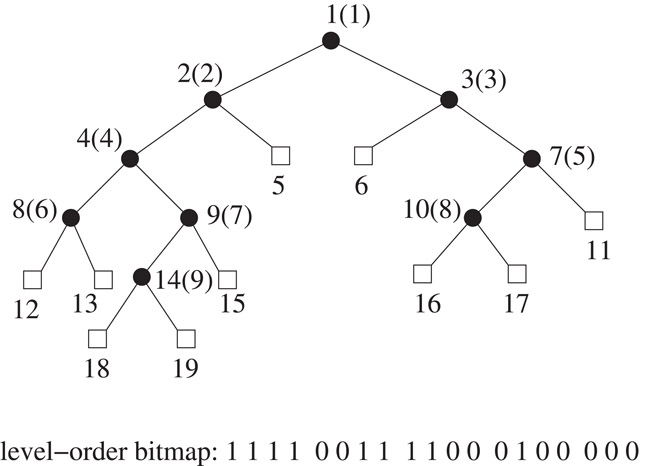
parent (i) = select (⌊ i / 2 ⌋); leftchild (i) = 2 \cdot rank (i); rightchild (i) = 2 \cdot rank (i) + 1.

$parent (i) = select (⌊ i / 2 ⌋); leftchild (i) = 2 \cdot rank (i); rightchild (i) = 2 \cdot rank (i) + 1.$

Figure 38.2Level-order bitmap representation of a binary tree.

38.4.2Ordinal Trees

Now, consider optimal representations of trees of higher degree, of which there are two different notions.

An ordinal tree is a rooted tree of arbitrary degree in which the children of each node are ordered. Ordinal trees on n nodes are in one to one correspondence with binary trees on n nodes. Hence about 2n bits are necessary to represent an arbitrary ordinal tree on n nodes. A cardinal tree of degree k is a rooted tree in which each node has k positions for an edge to a child. Hence, a binary tree is a cardinal tree of degree 2. There are $C_{n}^{k} \equiv (\binom{k n + 1}{n}) / (k n + 1)$ $C_{n}^{k} \equiv (\binom{k n + 1}{n}) / (k n + 1)$ cardinal trees of degree k on n nodes [20]. Hence we need roughly $(\lg (k - 1) + k \lg \frac{k}{(k - 1)}) n$ $(\lg (k - 1) + k \lg \frac{k}{(k - 1)}) n$ bits to represent an arbitrary such tree.

The basic operations we would like to support on tree representations are: given a node, finding its parent, ith child, degree and the size of the subtree rooted at that node (subtree size). For the cardinal trees we also need to support the additional operation of finding a child with a given label.

We outline three different representations of an ordinal tree. All the three representations map the n nodes of the tree onto the integers 1,…, n, and hence all are appropriate for applications in which data is to associated with nodes or leaves.

Level-order unary degree sequence representation: A rooted ordered tree can be represented by storing its degree sequence in any of a number of standard orderings of the nodes. The ordinal tree encoding of Jacobson [1] represents a node of degree d as a string of d 1s followed by a 0. Thus the degree of a node is represented by a binary prefix code. These prefix codes are then written in a level-order traversal of the entire tree. Using auxiliary structures to support rank and select operations on this sequence, one can support finding the parent, the ith child and the degree of any node in constant time. Thus, it gives a representation that takes 2n + o(n) bits of space and supports the above three operations in constant time, for an ordered tree on n nodes (Figure 38.3).

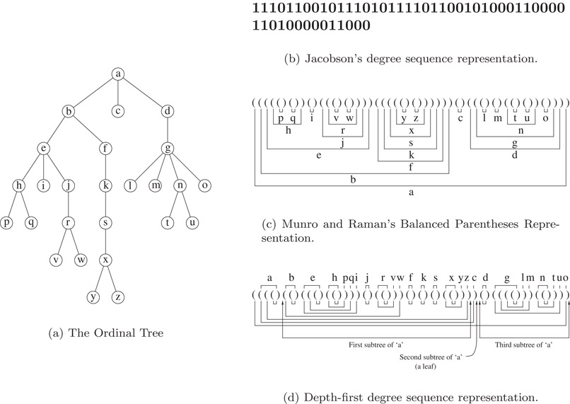
Figure 38.3Three encodings of an ordinal tree. (a) The Ordinal Tree, (b) Jacobson’s degree sequence representation, (c) Munro and Raman’s Balanced Parentheses Representation, (c) Depth-first degree sequence representation.

Balanced parenthesis representation: The tree encoding of Munro and Raman [21] uses a balanced sequence of parentheses to represent an ordinal tree. This balanced representation is derived from the depth-first traversal of the tree, writing an open parenthesis on the way down and a close parenthesis on the way up. Thus, a tree on n nodes can be represented by a balanced parenthesis sequence of length 2n. Extending the ideas of Jacobson, they showed how to support the following operations in O(1) time, using negligible extra space (o(n) bits):

•findopen/findclose(i): find the position of the open/close parenthesis matching the given close/open parenthesis in position i.

•excess(i): find the difference between the number of open and closing parentheses before the position i.

•enclose(i): given a parenthesis pair whose open parenthesis is in position i, find the open parenthesis corresponding to its closest enclosing matching parenthesis pair.

The parent of a node can be found in constant time using the enclose operation. In the parenthesis representation, the nodes of a subtree are stored together, which enables us to support the operation of finding the size of the subtree rooted at a given node in constant time. The problem with this representation is that finding the ith child takes Θ(i) time.

Depth-first unary degree sequence representation: Jacobson’s representation allows access to the ith child in constant time, whereas Munro and Raman’s representation supports subtree size operation in constant time. To combine the virtues of these two representations, Benoit et al. [22] used a representation that writes the unary degree sequence of each node in the depth-first traversal order of the tree. The representation of each node contains essentially the same information as in Jacobson’s level-order degree sequence, but written in a different order. Thus, it gives another 2n bit encoding of a tree on n nodes. Replacing the 0’s and 1’s by open and close parentheses respectively, and adding an extra open parenthesis at the beginning, creates a string of balanced parentheses. Using auxiliary structures to support rank and select operations on this bit string and also the operations on balanced parenthesis sequences defined above, one can support finding the parent, ith child, degree and subtree size of a given node in constant time.

Other operations: Sadakane [23] has shown that the parenthesis representation of an ordinal tree can be used to support least common ancestor queries in O(1) time using a o(n)-bit auxiliary structure. Munro and Rao [24] have shown that one can also support the level ancestor queries in O(1) time, using an additional o(n) bit auxiliary structure by storing the parenthesis representation. Geary et al. [25] obtained another structure that takes 2n + o(n) bits and supports level-ancestor queries, in addition to all the other navigational operations mentioned above in O(1) time.

38.4.3Cardinal Trees

A simple cardinal tree encoding can be obtained as follows: Encode each node of a k-ary tree by k bits, where the ith bit specifies whether child i is present. These can be written in any fixed ordering of the tree nodes, such as level order or depth-first order, to obtain the tree encoding. By storing the rank and select directories for this bitvector encoding, one can support parent, ith child and degree queries in constant time. This encoding has the major disadvantage of taking kn bits, far from the lower bound of roughly $(\lg k + \lg e) n$ $(\lg k + \lg e) n$ bits, as there are $C_{n}^{k} \equiv (\binom{k n + 1}{n}) / (k n + 1)$ $C_{n}^{k} \equiv (\binom{k n + 1}{n}) / (k n + 1)$ k-ary cardinal trees on n nodes.

Using some probabilistic assumptions, Darragh et al. [26] have implemented a structure that takes $\lg k + O (1)$ $\lg k + O (1)$ bits per node, though the implementation treats $\lg \lg n$ $\lg \lg n$ as “a constant” (indeed 5). This structure supports the navigational operations in constant expected time and also supports updates “efficiently” (compared with other linear space representations), and was also shown to perform well in practice.

To achieve a better space bound with good worst-case performance, one can use the ordinal tree encoding to store the underlying tree, and store some additional information about which children are present at each node. The ordinal information (using the depth-first unary degree sequence representation) can be used to support the parent, ith child, degree and subtree size queries in constant time.

Let S_x = {i1, i2,…, i_d} be the child labels of a node x with degree d in the cardinal tree. To find the child labeled j of node x, it suffices to find i = rank(j) in the set S_x, if j ∈ S_x. If i = − 1 (i.e., j ∉ S_x), then there is no child labeled j at node x, otherwise the ith child of x is the child labeled j of node x. The ith child can be found using the ordinal information. Storing each of these sets S_x using the indexable dictionary representation of Section 38.3.1, which takes $d \lg k + o (d) + O (\lg \lg k)$ $d \lg k + o (d) + O (\lg \lg k)$ bits for each S_x, requires $n \lg k + o (n) + O (n \lg \lg k)$ $n \lg k + o (n) + O (n \lg \lg k)$ bits in the worst case. Using a representation that stores a collection of indexable dictionaries efficiently [11], one can reduce the space consumption to $n \lg k + o (n) + O (\lg \lg k)$ $n \lg k + o (n) + O (\lg \lg k)$ bits.

Thus, this structure uses 2n + o(n) bits to represent the underlying ordinal tree, $n \lg k + o (n + \lg k)$ $n \lg k + o (n + \lg k)$ bits to represent the labels of the children at each node, and supports all the navigational operations and the subtree size operation in O(1) time.

Using the succinct indexable dictionary structure mentioned in Section 38.3, Raman et al. [11] obtained an optimal space cardinal tree representation. The main idea is to store the set of all pairs, $⟨ i, j ⟩$ $⟨ i, j ⟩$ such that the ith node, in the level-order of the nodes, has a child labeled j, using an indexable dictionary representation. (See Figure 38.4 for an example.) Since this set is of size n from the universe [nk], it requires $\lg (\binom{n k}{n}) + o (n + \lg k) = C_{n}^{k} + o (n + \lg k)$ $\lg (\binom{n k}{n}) + o (n + \lg k) = C_{n}^{k} + o (n + \lg k)$ bits to store an indexable dictionary for this set. One can easily map the navigational operations on the tree to the operations on this set, to support them in constant time. But this structure does not support the subtree size operation efficiently.

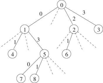
Figure 38.4The tree is represented by storing an indexable dictionary of the set ${⟨ 0, 0 ⟩, ⟨ 0, 2 ⟩, ⟨ 0, 3 ⟩, ⟨ 1, 1 ⟩, ⟨ 1, 3 ⟩, ⟨ 2, 1 ⟩, ⟨ 5, 0 ⟩, ⟨ 5, 1 ⟩}$ ${⟨ 0, 0 ⟩, ⟨ 0, 2 ⟩, ⟨ 0, 3 ⟩, ⟨ 1, 1 ⟩, ⟨ 1, 3 ⟩, ⟨ 2, 1 ⟩, ⟨ 5, 0 ⟩, ⟨ 5, 1 ⟩}$ .

38.4.4Dynamic Binary Trees

All the tree representations mentioned so far are static. Even to make a minor modification to the tree, such as adding a leaf, the entire structure has to be reconstructed (in the worst case). In this section we look at some representations that are more efficient in supporting updates to the tree.

Munro et al. [14] gave a binary tree representation that takes 2n + o(n) bits, and supports parent, left child, right child and subtree size operations in O(1) time. Updating the tree (adding a leaf or adding a node along an edge) requires $O (\lg^{c} n)$ $O (\lg^{c} n)$ time, for some constant c ≥ 1 which depends on the size of the data associated with the nodes. Extending some of the ideas involved in this, Raman and Rao [18] improved the update time to $O ((\lg \lg n)^{ϵ})$ $O ((\lg \lg n)^{ϵ})$ , for any fixed ε > 0, while maintaining the other time and space bounds (Figure 38.5).

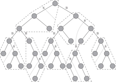
Figure 38.5Dynamic binary tree representation. B denotes an inter-block pointer and S denotes an inter-subblock pointer.

We briefly outline the key issues involved in the construction of these structures. First, we divide the tree into blocks of size $Θ (\lg^{c} n)$ $Θ (\lg^{c} n)$ , for some c ≥ 2, and each block in turn into sub-blocks of size $ϵ \lg n$ $ϵ \lg n$ , for some fixed ε < 1. The sub-blocks are stored using an implicit representation and are operated upon using precomputed tables. The block structure of the tree is stored using explicit pointers. Since there are only $Θ (\lg^{c - 1} n)$ $Θ (\lg^{c - 1} n)$ sub-blocks in each block, we can store the sub-block structure within a block explicitly using $Θ (\lg \lg n)$ $Θ (\lg \lg n)$ sized pointers. Each block stores its parent block and the size, using a constant number of words. Thus, the overall block structure of the tree is easily handled by conventional means (storing explicit pointers) and only takes $O (n / \lg n)$ $O (n / \lg n)$ bits. The blocks and sub-blocks tolerate some slack in their sizes and are moved to appropriate sized areas to avoid wasting space. Ultimately, the key issues boil down to the memory management.

To support subtree size, we maintain the the subtree sizes of the roots of all blocks and sub-blocks. Since each update changes the subtree sizes of several nodes, it is not possible to update all the effected blocks and sub-blocks in constant time, in general. For this reason, we assume that the navigation through the tree begins at the root and may end at any point (or at the root, to achieve worst-case constant time for updates), and navigates the tree by moving from a node only to either its parent or one of its children. Hence, updates to a node higher in the tree regarding the insertions and deletions to descendants are made on return to that node.

38.5Graph Representations

In this section, we briefly describe some space efficient representations of graphs. In particular, we consider representations that take close to the information theoretic minimum space and support degree and adjacency queries efficiently. A degree query asks for the degree of a given node in the graph, and an adjacency query asks whether two given vertices are adjacent or not in the graph. In addition, we would also like to support listing all the vertices adjacent to a given vertex.

Turán [27] gave a linear time constructible representation of an arbitrary planar graph that takes at most 12 bits per node. Though this gives a space efficient representation of planar graphs, it does not support the queries efficiently. Kannan et al. [28] have given an implicit (linear space) graph representation that supports adjacency queries using $O (\lg n)$ $O (\lg n)$ bit probes.

Jacobson [1] gave a representation that takes O(n) bits of space to represent a planar graph on n nodes and supports degree and adjacency queries in constant time. It uses a simple mapping of one-page graphs to sequences of balanced parentheses, and the fact that a planar graph always has a 4-page embedding. By storing auxiliary structures to support some natural operations on these sequences (see Section 38.4.2), one can also support the navigational operations in optimal time.

Munro and Raman [21] improved the space to 8n + 2m + o(n) bits, for a planar graph on n vertices with m edges, still supporting the queries in constant time. In general, their representation takes 2kn + 2m + o(nk + m) bits to store a k page graph on n vertices and m edges and supports degree and adjacency queries in O(k) time.

There have been several improvements [29–33], improving the space close to the information theoretic-lower bound, simultaneously expanding the class of graphs for which the scheme works. In particular, Lu [33] gave an optimal space (within lower-order terms) representation that can be constructed in linear time. This supports degree and adjacency queries in O(1) time for constant-genus graphs.

The main idea is to partition the given graph G on n vertices into $o (n / \lg n)$ $o (n / \lg n)$ disjoint subgraphs of size $O (\lg^{6} n)$ $O (\lg^{6} n)$ by removing a subgraph H of size $o (n / \lg n)$ $o (n / \lg n)$ . This is done using a “planarization algorithm” for bounded genus graphs, and an algorithm to construct a “separator decomposition tree” of a planar graph. The representation of G is obtained by storing a rerepresentation of H, and recursing on each of the smaller subgraphs upto a constant number of levels, after which one can use a precomputed table to operate on the small subgraphs. See [33] for details.

38.6Succinct Structures for Indexing

A text index is a data structure storing a text (a string or a set of strings) and supporting string matching queries: given a pattern P, find all the occurrences of P in the text. Two well-known and widely used index structures are the suffix trees and suffix arrays. In this section we briefly describe some succinct data structures for these two.

A suffix tree for a text is the compressed digital trie of all the suffixes of the text [34,35]. A suffix tree for a text of length n has n leaves and at most n − 1 internal nodes. The space bound is a consequence of skipping nodes with only one child, hence there are precisely n − 1 internal nodes if we use a binary trie. Each leaf points to the position in the text of the corresponding suffix it represents uniquely. The edges are labeled by substrings of the text, which are usually represented by storing a position in the text where the substring starts and its length. Thus, a standard representation of a suffix tree for a text of length n takes $O (n \lg n)$ $O (n \lg n)$ bits. Searching for an occurrence of a pattern of length m using a suffix tree takes O(m) time.

The suffix array of a text is an array storing pointers to the suffixes of the text in their lexicographic order. Thus, a suffix array for a text of length n takes $n ⌈ \lg n ⌉$ $n ⌈ \lg n ⌉$ bits. Note that the leaf labels of a suffix tree written from left to right form the suffix array, if the children of each node are arranged in lexicographic order of their edge labels. Searching for an occurrence of a pattern of length m using a suffix array takes $O (m + \lg n)$ $O (m + \lg n)$ time.

We now briefly sketch the ideas involved in representing a suffix tree (and hence also a suffix array) using O(n) bits. We first convert the trie into binary by using a fixed length encoding of the characters of the alphabet. We then store the parenthesis representation of the underlying tree structure (see Section 38.4.2). The edge labels of a suffix tree can be omitted, as this can be determined by finding the longest common prefix of the leftmost and rightmost leaves of the parent node (of the edge). The parenthesis representation of an ordinal tree can be augmented with o(n)-bit additional structure to support finding the leftmost and rightmost leaves of a given node in constant time. Thus, one can use this tree representation to store the tree structure of a suffix tree, and store the leaf pointers (suffix array) explicitly. This gives a suffix tree representation that takes $n \lg n + O (n)$ $n \lg n + O (n)$ bits of space and supports indexing queries in optimal time. See [4] for details.

The above structure uses $n ⌈ \lg n ⌉$ $n ⌈ \lg n ⌉$ bits to represent the pointers to the text or the suffix array. Grossi and Vitter [36] obtained a suffix array structure that takes O(n) bits and supports finding the ith element in the suffix array (lookup queries) in $O (\lg^{ϵ} n)$ $O (\lg^{ϵ} n)$ time, for any fixed ε > 0. Using this structure they also obtained a suffix tree representation that takes O(n) bits of space and supports finding all the s occurrences of a given pattern of length m in $O (m + s \lg^{ϵ} n)$ $O (m + s \lg^{ϵ} n)$ time. The structure given by Rao [37] generalizes the suffix array structure of Grossi and Vitter, which takes $O (n t (\lg n)^{1 / (t + 1)})$ $O (n t (\lg n)^{1 / (t + 1)})$ bits and supports lookup in O(t) time, for any parameter $1 \leq t \leq \lg \lg n$ $1 \leq t \leq \lg \lg n$ . Using this structure, one can get an index structure that takes $o (n \lg n)$ $o (n \lg n)$ bits and supports finding all the s occurrences of a given pattern of length m in $O (m + s + \lg^{ϵ} n)$ $O (m + s + \lg^{ϵ} n)$ time.

Ferragina and Manzini [38] presented an opportunistic data structure taking O(nH_k(n)) + o(n) bits of space, where H_k(n) denotes the kth order entropy of the given text of length n. This supports finding all the occurrences of a pattern of length m in $O ((m + s) \lg^{ϵ} n)$ $O ((m + s) \lg^{ϵ} n)$ time, where s is the number of occurrences of the pattern. They also presented its practical performance [39].

Sadakane [23] gave a data structure that takes $O (n \cdot (1 + H_{0}) + O (| Σ | \lg | Σ |))$ $O (n \cdot (1 + H_{0}) + O (| Σ | \lg | Σ |))$ bits for a text of length n over an alphabet Σ, where $H_{0} \leq \lg | Σ |$ $H_{0} \leq \lg | Σ |$ is the order-0 entropy for the text. This supports finding all the s occurrences of a given pattern P in $O (| P | \lg n + s \lg^{ϵ} n)$ $O (| P | \lg n + s \lg^{ϵ} n)$ time, and decompress a portion of the text of length l in $O (l + \lg^{ϵ} n)$ $O (l + \lg^{ϵ} n)$ time, for any fixed ε > 0.

Grossi et al. [40] gave another index structure that takes $n H_{k} (n) + O (n \lg \lg n \lg | Σ | / \lg n)$ $n H_{k} (n) + O (n \lg \lg n \lg | Σ | / \lg n)$ bits for a text of length n over an alphabet Σ. Finding an occurrence of a pattern of length m using this structure takes $O (m \lg | Σ | + p o l y l o g (n))$ $O (m \lg | Σ | + p o l y l o g (n))$ time. This is also shown to perform well, in terms of space as well as query times, in practice [41].

38.7Permutations and Functions

38.7.1Permutations

Permutations are fundamental in computer science and have been the focus of extensive study. Here we consider the problem of representing permutations succinctly to support computing πk(i) for any integer k, where π0(i) = i for all i; πk(i) = π(π^{k − 1}(i)) when k > 0 and πk(i) = π^{− 1}(π^{k + 1}(i)) when k < 0.

The most obvious way of representing an arbitrary permutation, π, of the integers {0,1,…, n − 1} is to store the sequence π(0), π(1),…, π(n − 1). This takes $n ⌈ \lg n ⌉$ $n ⌈ \lg n ⌉$ bits, which is Θ(n) bits more than the information-theoretic lower bound of $\lg (n!) \approx n \lg n - n \lg e$ $\lg (n!) \approx n \lg n - n \lg e$ bits. This representation can be used to find π(i) in O(1) time, but finding π⁻¹(i) takes O(n) time in the worst case, for 0 ≤ i ≤ n − 1. Using this representation, one can easily compute πk(i) in k steps, for k ≥ 1. To facilitate the computation in constant time, one could store πk(i) for all i and k (|k| ≤ n, along with its cycle length), but that would require $Θ (n^{2} \lg n)$ $Θ (n^{2} \lg n)$ bits. The most natural compromise is to retain πk(i) with |k| ≤ n a power of 2. Unfortunately, this $n ⌈ {\lg n}^{2} ⌉$ $n ⌈ {\lg n}^{2} ⌉$ bit representation leaves us with a logarithmic time evaluation scheme and a factor of $\lg n$ $\lg n$ from the minimal space representation.

We first show how to augment the standard representation to support π⁻¹ queries efficiently, while avoiding most of the extra storage cost one would expect. In addition to storing the standard representation, we trace the cycle structure of the permutation, and for every cycle whose length is at least t, we store a shortcut pointer with the elements which are at a distance of a multiple of t steps from an arbitrary starting point. The shortcut pointer points to the element which is t steps before it in the cycle of the permutation. This shortcut representation of a permutation can be stored using $(1 + 1 / t) n \lg n + o (n)$ $(1 + 1 / t) n \lg n + o (n)$ bits, and it supports π queries in O(1) time and π⁻¹ queries in O(t) time, for any parameter 1 ≤ t ≤ n.

Consider the cycle representation of a permutation π over {0, 1,…, n − 1}, which is a collection of disjoint cycles of π (where the cycles are ordered arbitrarily). Let σ be this permutation, that is, the standard representation of σ is a cycle representation of π. Let B be a bit vector of length n that has a 1 corresponding to the starting position of each cycle of π and 0 everywhere else, together with its rank and select directories with respect to both bits. Let S be a representation of σ that supports σ(i) and σ^{− 1}(i) queries efficiently. Then to find πk(i), first find the index j of the cycle to which σ⁻¹(i) belongs, using B and S. Find the length l of the jth cycle and the number p of elements up to (but not including) the jth cycle. Then, one can verify that πk(i) = σ(p + (i − p + k mod l)). Combining this with the shortcut representation, one can get a representation taking $(1 + ϵ) n \lg n + O (1)$ $(1 + ϵ) n \lg n + O (1)$ bits that supports computing arbitrary powers in O(1) time.

Benes network: A Benes network [42] is a communication network composed of a number of switches. Each switch has 2 inputs x0 and x1 and 2 outputs y0 and y1 and can be configured either so that x0 is connected to y0 (i.e., a packet that is input along x0 comes out of y0) and x1 is connected to y1, or the other way around. An r-Benes network has 2r inputs and outputs, and is defined as follows. For r = 1, the Benes network is a single switch with 2 inputs and 2 outputs. An (r + 1)-Benes network is composed of 2^{r + 1} switches and two r-Benes networks, connected as as shown in Figure 38.6a. A particular setting of the switches of a Benes network realizes a permutation π if a packet introduced at input i comes out at output π(i), for all i. See Figure 38.6b for an example.

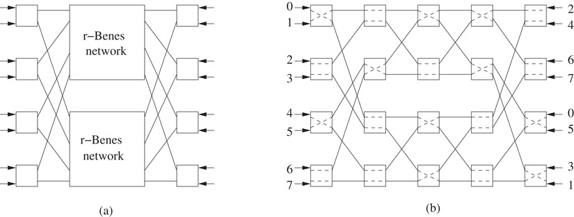
Figure 38.6Benes network: (a) construction of (r + 1)-Benes network (b) Benes network realizing the permutation (4,7,0,6,1,5,2,3).

Clearly, a Benes network may be used to represent a permutation. For example, if n = 2r, a representation of a permutation π on [n] may be obtained by configuring an r-Benes network to realize π and then listing the settings of the switches in some canonical order (e.g., level-order). This represents π using r2r − 2^{r − 1} = $n \lg n - n / 2$ $n \lg n - n / 2$ bits. Given i, one can trace the path taken by a packet at input i by inspecting the appropriate bits in this representation, and thereby calculate π(i) in $O (\lg n)$ $O (\lg n)$ time (indeed, in $O (\lg n)$ $O (\lg n)$ bit-probes). In fact, by tracing the path back from output i we can also compute π⁻¹(i) in $O (\lg n)$ $O (\lg n)$ time.

One can compress the middle levels of a Benes network by storing an implicit representation of the permutation represented by the middle $O (\lg n / \lg \lg n)$ $O (\lg n / \lg \lg n)$ levels. This reduces the space to $\lg (n!) + o (n)$ $\lg (n!) + o (n)$ bits. One can also group the remaining bits of this Benes network into words of size $Θ (\lg n)$ $Θ (\lg n)$ bits (by taking $O (\lg \lg n)$ $O (\lg \lg n)$ consecutive levels and $O (\lg \lg n)$ $O (\lg \lg n)$ appropriate rows). This enables us to traverse $Θ (\lg \lg n)$ $Θ (\lg \lg n)$ levels in a Benes network in O(1) time. Thus, it gives a representation that takes the optimal $⌈ \lg (n!) ⌉ + o (n)$ $⌈ \lg (n!) ⌉ + o (n)$ bits, and supports computing arbitrary powers in $O (\lg n / \lg \lg n)$ $O (\lg n / \lg \lg n)$ time.

One can obtain a structure with same time and space bounds even when n is not a power of 2. See [43] for details.

38.7.2Functions

Now consider the problem of representing arbitrary functions $f : [n] \to [n]$ $f : [n] \to [n]$ , so that queries for fk(i), for any integer k can be answered efficiently. Here f0(i) = i and for any k > 0, fk(i) = f(f^{k −1}(i)) and f^{− k}(i) = {j|fk(j) = i}, for all i. This is a generalization of the problem considered in the previous section. Since there are nn functions from [n] to [n], any representation scheme takes at least $⌈ n \lg n ⌉$ $⌈ n \lg n ⌉$ bits to store an arbitrary function.

A standard way of representing a function is to store the sequence f(i), for i = 0,…, n − 1. This representation does not support the efficient evaluation of fk(i) for k≫1. We look at a representation that takes $(1 + ϵ) n \lg n + O (1)$ $(1 + ϵ) n \lg n + O (1)$ bits of space to store a function $f : [n] \to [n]$ $f : [n] \to [n]$ and supports computing arbitrary positive powers in constant time and negative powers f^{− k}(i), in O(1 + |f^{− k}(i)|) time.

Given an arbitrary function $f : [n] \to [n]$ $f : [n] \to [n]$ , consider the directed graph, G_f = (V, E), obtained from it, where V = [n] and E = {(i, j):f(i) = j}. In general this directed graph consists of a disjoint set of subgraphs, each of which is a directed cycle with trees rooted at the nodes on the cycle and edges directed towards the roots. See Figure 38.7 for an example.

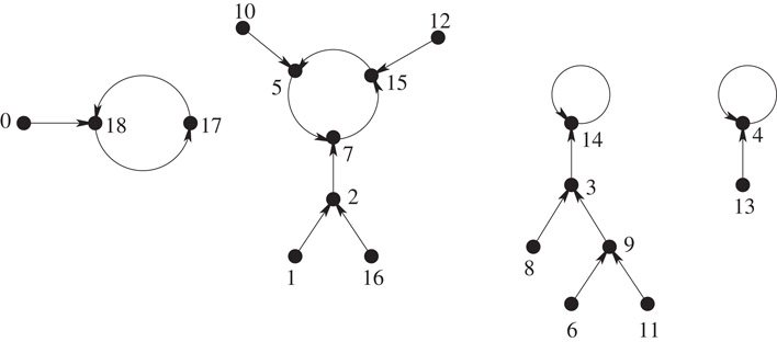
Figure 38.7Graph representation of the function f(x) = (x2 + 2x − 1) mod 19, for 0 ≤ x ≤ 18.

The main idea of the solution is as follows: in each directed cycle, we re-order the nodes of each tree such that the leftmost path of any subtree is the longest path in that subtree. This enables finding a node at a given depth from any internal node, if it exists, in constant time using the parenthesis representation. We then preprocess each of the trees and store auxiliary structures to support level-ancestor queries on them in constant time (see Section 38.4.2). Observe that finding fk(i), for k > 0, can be translated to finding the ancestor of node i which is k levels above it, if i is at a depth at least k in its tree T. Otherwise, we have to traverse the cycle to which the root of T belongs, to find the required answer. This can be done by storing these cycles as a permutation.

When i belongs to one of the trees in a subgraph, one can answer fk(i) queries for k < 0 in optimal time by finding all the nodes that are at the kth level in the subtree rooted at i. Otherwise, if i is part of the cycle in the subgraph, we store an auxiliary structure that, for any given i and k, outputs all the trees in the subgraph containing i that have an answer in time proportional to the number of such nodes. From this, one can easily find the required answer in optimal time. The auxiliary structure takes O(m) bits for a subgraph with m nodes, and hence O(n) bits overall. See [24] for details.

For functions from $[n] \to [m]$ $[n] \to [m]$ one can show the following: If there is a representation of a permutation that takes P(n) space to represent a permutation on [n] and supports forward in t1 time and inverse in t2 time, then there is a representation of a function from [n] to [m], m ≤ n that takes $(n - m) \lg m + P (m) + O (m)$ $(n - m) \lg m + P (m) + O (m)$ bits, and supports fk(i) in O(t1 + t2) time, for any positive integer k and for any i ∈ [n]. When m > n, larger powers are not defined in general. In this case, we can have a structure that takes $n \lg m + P (n) + O (n)$ $n \lg m + P (n) + O (n)$ bits of space and answers queries for positive powers (returns the power if defined or returns − 1 otherwise) in O(t1 + t2) time.

38.8Partial Sums

Let a1, a2,…, a_n be a sequence of n non-negative k-bit numbers. The partial sums problem maintains the sequence under the following operations:

•sum(i): return $\sum_{j = 1}^{i} a_{j}$ $\sum_{j = 1}^{i} a_{j}$ ,

•update(i, δ): set $a_{i} \leftarrow a_{i} + δ$ $a_{i} \leftarrow a_{i} + δ$ , for some integer δ such that 0 ≤ a_i + δ ≤ 2k − 1. Our later solutions have the additional constraint that $| δ | \leq \lg^{O (1)} n$ $| δ | \leq \lg^{O (1)} n$ .

Dietz [44] gave a structure for the partial sum problem that supports sum and update in $O (\lg n / \lg \lg n)$ $O (\lg n / \lg \lg n)$ time using $O (n \lg n)$ $O (n \lg n)$ bits of extra space, for the case when $k = Θ (\lg n)$ $k = Θ (\lg n)$ and no constraints on δ. The time bounds are optimal due to the lower bound of Fredman and Saks [45]. As the information-theoretic space lower bound is kn bits, this structure uses space within a constant factor of the optimal.

The main idea of this structure is to store the elements at the leaves of a complete tree with branching factor $O (\lg^{ϵ} n)$ $O (\lg^{ϵ} n)$ for some ε < 1. The operations are performed by traversing a path from a leaf to the root, querying/updating the nodes along the path.

The searchable partial sums problem is an extension of the partial sums problem that also supports the following operation:

•search(j): find the smallest i such that sum(i) ≥ j.

When k = 1 (i.e., each element is a bit), the special case is commonly known as the dynamic bit vector problem, which maintains a bit vector of length n under rank, select and flip (update) operations.

For the searchable partial sums problem there is a structure that supports all operations in $O (\lg n / \lg \lg n)$ $O (\lg n / \lg \lg n)$ time, and uses kn + o(kn) bits of space [46]. For $k = O (\lg \lg n)$ $k = O (\lg \lg n)$ , one can also obtain a structure that again takes kn + o(kn) bits and supports sum and search in O(log_b n) time and update in O(b) amortized time, for any parameter $b \geq \lg n / \lg \lg n$ $b \geq \lg n / \lg \lg n$ [47]. For the partial sums problem, one can support the above trade-off for $k = O (\lg n)$ $k = O (\lg n)$ [46], and the time bounds can be shown to be optimal [45].

For the dynamic bit vector problem, one can support rank and select in O(log_b n) time and flip in O(b) (worst-case) time, for any parameter $\lg n / \lg \lg n \leq b \leq n$ $\lg n / \lg \lg n \leq b \leq n$ , using o(n) bits of extra space. One can also extend the above trade-off for $k = O (\lg \lg n)$ $k = O (\lg \lg n)$ , using kn + o(kn) bits of space.

See [46,47] for details.

38.9Arrays

38.9.1Resizable Arrays

A basic problem that arises in many applications is accumulating elements into a list when the number of elements is unknown ahead of time. The operations needed from such a structure are the ability to append elements to the end of the structure, removing the last element from the structure (in applications such as implementing a stack) and some method of accessing the elements currently in the structure.

One simple solution is a linked list which can easily grow and shrink, and supports sequential access. But this does not support random access to the elements. Moreover, its space overhead is O(n) pointers to store n elements.

Another standard solution is the doubling technique [48]. Here the elements are stored in an array. Whenever the array becomes full, an array of double its size allocated and all the elements are copied to it. Similarly, whenever the array shrinks so that it is only one-fourth full, an array of half its size is allocated and all the elements are copied to it. The advantage of this solution over the linked lists is that random access to the elements takes only O(1) time (as opposed to O(n) for linked lists). The amortized update time is O(1), though the worst-case update time is O(n). The space overhead of this solution is O(n).

Sitarski [49] has proposed a solution whose space overhead is only $O (\sqrt{n})$ $O (\sqrt{n})$ . The idea is to divide the given list of n elements into sublists of size $⌈ \sqrt{n} ⌉$ $⌈ \sqrt{n} ⌉$ , store them in separate arrays, and store an array (of length $O (\sqrt{n})$ $O (\sqrt{n})$ ) of pointers to these sublists (in order). Whenever $⌈ \sqrt{n} ⌉$ $⌈ \sqrt{n} ⌉$ changes, the entire structure is reconstructed with the new size. Thus the amortized update time is O(1) (though the worst-case time is O(n)). This also supports random access in O(1) time.

Brodnik et al. [13] gave a structure that takes $O (\sqrt{n})$ $O (\sqrt{n})$ extra locations, where n is the current size of the array, and supports the operations in O(1) time. One advantage of this structure is that elements are never re-allocated. They have also shown that any such structure requires $Ω (\sqrt{n})$ $Ω (\sqrt{n})$ extra locations even if there are no constraints on the access time.

38.9.2Dynamic Arrays

A resizable array supports adding/deleting elements only at the end of the list, but does not support insertion/deletion of elements at arbitrary positions in the array. A dynamic array is data structure that maintains a sequence of records under the following operations:

•access(i): return the ith record in the sequence,

•insert(r, i): insert the record r at position i in the sequence, and

•delete(i): delete the ith record in the sequence.

A standard way of implementing a dynamic array is to store the records in an array and maintain it using the doubling technique. This supports access in O(1) but requires O(n) time to support insert and delete operations.

Goodrich and Kloss [50] gave a structure, the tiered vector, that takes $n + O (\sqrt{n})$ $n + O (\sqrt{n})$ words of space to represent a sequence of length n, where each record fits in a word. This structure supports access in O(1) time and updates in $O (\sqrt{n})$ $O (\sqrt{n})$ amortized time. The major component of a tiered vector is a set of indexable circular deques. A deque is a linear list which provides constant time insert and delete operations at either the head or the tail of the list [51]. A circular deque is a list which is stored in a sequential section of memory of fixed size. An indexable circular deque maintains pointers h and t, which reference the index in memory of the head and tail of this list. A tiered vector is a set of indexable circular deques. Insertions and deletions in an arbitrary indexable circular deque require time linear in its size, but inserting/deleting at either the head or the tail of the list takes O(1) time.

Thus, by maintaining the given sequence of n elements using $O (\sqrt{n})$ $O (\sqrt{n})$ indexable circular deques each of size $O (\sqrt{n})$ $O (\sqrt{n})$ , one can support access in O(1) time and updates in $O (\sqrt{n})$ $O (\sqrt{n})$ amortized time. One can easily generalize this structure to one that supports access in O(1/ε) time and updates in O(n^ε) time, for any parameter 0 < ε ≤ 1.

Using this structure to represent a block of $O (\lg^{O (1)} n)$ $O (\lg^{O (1)} n)$ records, Raman et al. [46] gave a structure that supports access and updates in $O (\lg n / \lg \lg n)$ $O (\lg n / \lg \lg n)$ amortized time, using o(n) bits of extra space. The main idea is to divide the given list of length n into sublists of length between $(1 / 2) \lg^{4} n$ $(1 / 2) \lg^{4} n$ and $2 \lg^{4} n$ $2 \lg^{4} n$ , and store the sublists using the above dynamic array structure. One can maintain these sublists as the leaves of a weight-balanced B-tree with branching factor $O (\sqrt{\lg n})$ $O (\sqrt{\lg n})$ , and hence height $O (\lg n / \lg \lg n)$ $O (\lg n / \lg \lg n)$ .

By restricting the length of the array, Raman and Rao [18] obtained a dynamic array structure that maintains a sequence of l = O(w^O(1)) records of r = O(w) bits each, where w is the word size. This structure supports access in O(1) time and updates in O(1 + lr/kw) amortized time, and uses $l r + O (k \lg l)$ $l r + O (k \lg l)$ bits, for any parameter k ≤ l. The data structure also requires a precomputed table of size O(2^εw) bits, for any fixed ε > 0. The main idea is to store the newly added elements separately from the existing elements, and store a structure to indicate all the positions of the “updated” elements. The structure is rebuilt after every k updates.

38.10Conclusions

We looked at several succinct data structures that achieve almost optimal space while supporting the required operations efficiently. Apart from being of theoretical interest, succinct data structures will also have many practical applications due to the enormous growth in the amount of data that needs to be stored in a structured fashion.

Most of the succinct data structures we presented here can be constructed in linear time from the standard representation. But this method requires more space than necessary during the construction. Developing algorithms that directly construct the succinct representations without using more space during construction, preferably in optimal time, is an important open problem. See [52] for an example.

Another aspect, that is more of theoretical significance, is to study the cell probe (in particular, bit probe) complexity of succinct data structures [53–55]. For most problems, no bounds other than the straightforward translations from the bounds on the RAM model are known. It is also interesting to consider the time-space trade-offs of these structures.

References

1.G. Jacobson. Succinct Static Data Structures. PhD thesis, Carnegie Mellon University, 1988.

2.J. Ian Munro. Tables. Proceedings of the Conference on Foundations of Software Technology and Theoretical Computer Science, LNCS 1180: 37–42, 1996.

3.D. R. Clark. Compact Pat Trees. PhD thesis, University of Waterloo, 1996.

4.J. Ian Munro, V. Raman, and S. Srinivasa Rao. Space Efficient Suffix trees. Journal of Algorithms, 39(2): 205–222, 2001.

5.M. L. Fredman, J. Komlós, and E. Szemerédi. Storing a Sparse Table with O(1) Worst Case Access Time. Journal of the ACM, 31(3): 538–544, 1984.

6.J. P. Schmidt and A. Siegel. The Spatial Complexity of Oblivious k-probe Hash Functions. SIAM Journal on Computing, 19(5): 775–786, 1990.

7.A. Brodnik and J. Ian Munro. Membership in Constant Time and Almost Minimum Space. SIAM Journal on Computing, 28(5): 1627–1640, 1999.

8.R. Pagh. Low Redundancy in Static Dictionaries with Constant Query Time. SIAM Journal on Computing, 31(2): 353–363, 2001.

9.M. Ajtai. A Lower Bound for Finding Predecessors in Yao’s Cell Probe Model. Combinatorica, 8(3): 235–247, 1988.

10.V. Raman and S. Srinivasa Rao. Static Dictionaries Supporting Rank. Proceedings of the International Symposium on Algorithms and Computation, LNCS 1741: 18–26, 1999.

11.R. Raman, V. Raman, and S. Srinivasa Rao. Succinct Indexable Dictionaries with Applications to Encoding k-ary Trees and Multisets. Proceedings of the ACM-SIAM Symposium on Discrete Algorithms, 233–242, 2002.

12.P. Elias. Efficient Storage and Retrieval by Content and Address of Static Files. Journal of the ACM, 21(2): 246–260, 1974.

13.A. Brodnik, S. Carlsson, E. D. Demaine, J. Ian Munro, and R. Sedgewick. Resizable Arrays in Optimal Time and Space. Proceedings of the Workshop on Algorithms and Data Structures, LNCS 1663: 37–48, 1999.

14.J. Ian Munro, V. Raman, and A. Storm. Representing Dynamic Binary Trees Succinctly. Proceedings of the ACM-SIAM Symposium on Discrete Algorithms, 529–536, 2001.

15.M. Dietzfelbinger, A. R. Karlin, K. Mehlhorn, F. Meyer auf der Heide, H. Rohnert, and R. E. Tarjan. Dynamic Perfect Hashing: Upper and Lower Bounds. SIAM Journal on Computing, 23(4): 738–761, 1994.

16.R. Pagh and F. F. Rodler. Cuckoo Hashing. Proceedings of the European Symposium on Algorithms, LNCS 2161: 121–133, 2001.

17.D. Fotakis, R. Pagh, P. Sanders, and P. G. Spirakis. Space Efficient Hash Tables with Worst Case Constant Access Time. Proceedings of Symposium on Theoretical Aspects of Computer Science, LNCS 2607: 271–282, 2003.

18.R. Raman and S. Srinivasa Rao. Dynamic Dictionaries and Binary Trees in Near-minimum Space. Proceedings of the International Colloquium on Automata, Languages and Programming, LNCS 2719: 357–368, 2003.

19.J. W. J. Williams. Algorithm 232: Heap Sort. Communications of the ACM, 7(6): 347–348, 1964.

20.R. L. Graham, D. E. Knuth, and O. Patashnik. Concrete Mathematics. Addison-Wesley, 1989.

21.J. Ian Munro and V. Raman. Succinct Representation of Balanced Parentheses and Static Trees. SIAM Journal on Computing, 31(3): 762–776, 2001.

22.D. Benoit, E. D. Demaine, J. Ian Munro, and V. Raman. Representing Trees of Higher Degree. Proceedings of the Workshop on Algorithms and Data Structures, LNCS 1663: 169–180, 1999.

23.K. Sadakane. Succinct Representations of lcp Information and Improvements in the Compressed Suffix Arrays. Proceedings of the ACM-SIAM Symposium on Discrete Algorithms, 225–232, 2002.

24.J. Ian Munro and S. Srinivasa Rao. Succinct Representations of Functions. Proceedings of the International Colloquium on Automata, Languages and programming, LNCS 3142, 1006–1015, 2004.

25.R. F. Geary, R. Raman, and V. Raman. Succinct Ordinal Trees with Level-ancestor Queries. Proceedings of the ACM-SIAM Symposium on Discrete Algorithms, 1–10, 2004.

26.J. J. Darragh, J. G. Cleary, and I. H. Witten. Bonsai: A Compact Representation of Trees. Software Practice and Experience, 23(3): 277–291, 1993.

27.G. Turán. Succinct Representations of Graphs. Discrete Applied Mathematics, 8: 289–294, 1984.

28.S. Kannan, M. Naor, and S. Rudich. Implicit Representation of Graphs. Proceedings of the ACM Symposium on Theory of Computing, 334–343, 1988.

29.R. C. Chuang, A. Garg, X. He, M.-Y. Kao, and H.-I. Lu. Compact Encodings of Planar Graphs via Canonical Orderings and Multiple Parentheses. Proceedings of the International Colloquium on Automata, Languages and Programming, LNCS 1443: 118–129, 1998.

30.Y.-T. Chiang, C.-C. Lin, and H.-I. Lu. Orderly Spanning Trees with Applications to Graph Drawing and Graph Encoding. Proceedings of the ACM-SIAM Symposium on Discrete Algorithms, 506–515, 2001.

31.X. He, M.-Y. Kao, and H.-I. Lu. Linear-time Succinct Encodings of Planar Graphs via Canonical Orderings. SIAM Journal on Discrete Mathematics, 12: 317–325, 1999.

32.H.-I. Lu. Linear-time Compression of Bounded-genus Graphs into Information-theoretically Optimal Number of Bits. Proceedings of the ACM-SIAM Symposium on Discrete Algorithms, 223–224, 2002.

33.H.-I. Lu. Linear-Time Information-theoretically Optimal Encodings Supporting Constant-time Queries for Constant-genus Graphs. Manuscript, 2002.

34.P. Weiner. Linear Pattern Matching Algorithm. Proceedings of the IEEE Symposium on Switching and Automata Theory, 1–11, 1973.

35.E. M. McCreight. A Space-economical Suffix Tree Construction Algorithm. Journal of the ACM, 23(2): 262–272, 1976.

36.R. Grossi and J. S. Vitter. Compressed Suffix Arrays and Suffix Trees with Applications to Text Indexing and String Matching. Proceedings of the ACM Symposium on Theory of Computing, 397–406, 2000.

37.S. Srinivasa Rao. Time Space Tradeoffs for Compressed Suffix Arrays. Information Processing Letters, 82(6): 307–311, 2002.

38.P. Ferragina and G. Manzini. Opportunistic Data Structures with Applications. Proceedings of the Annual Symposium on Foundations of Computer Science, 390–398, 2000.

39.P. Ferragina and G. Manzini. An Experimental Study of an Opportunistic Index. Proceedings of the Annual Symposium on Foundations of Computer Science, 269–278, 2001.

40.R. Grossi, A. Gupta, and J. S. Vitter. High-order Entropy-compressed Text Indexes. Proceedings of the ACM-SIAM Symposium on Discrete Algorithms, 841–850, 2003.

41.R. Grossi, A. Gupta, and J. S. Vitter. When Indexing Equals Compression: Experiments with Compressing Suffix Arrays and Applications. Proceedings of the ACM-SIAM Symposium on Discrete Algorithms, 629–638, 2004.

42.F. T. Leighton. Introduction to Parallel Algorithms and Architectures: Arrays, Trees and Hypercubes. Computer Science and Information Processing, Morgan Kauffman, 1992.

43.J. Ian Munro, V. Raman, R. Raman, and S. Srinivasa Rao. Succinct Representations of Permutations. Proceedings of the International Colloquium on Automata, Languages and Programming, LNCS 2719: 345–356, 2003.

44.P. F. Dietz. Optimal Algorithms for List Indexing and List Ranking. Proceedings of the Workshop on Algorithms and Data Structures, LNCS 382: 39–46, 1989.

45.M. L. Fredman and M. E. Saks. The Cell Probe Complexity of Dynamic Data Structures. Proceedings of the ACM Symposium on Theory of Computing, 345–354, 1989.

46.R. Raman, V. Raman, and S. Srinivasa Rao. Succinct Dynamic Data Structures. Proceedings of the Workshop on Algorithms and Data Structures, LNCS 2125, 426–437, 2001.

47.W.-K. Hon, K. Sadakane, and W.-K. Sung. Succinct Data Structures for Searchable Partial Sums. Proceedings of the International Symposium on Algorithms and Computation, LNCS 2906, 505–516, 2003.

48.J. Boyer. Algorithm Alley: Resizable Data Structures. Dr. Dobb’s Journal, 23(1), January 1998.

49.E. Sitarski. Algorithm Alley: HATs: Hashed Array Tables. Dr. Dobb’s Journal, 21(11), September 1996.

50.M. T. Goodrich and J. G. Kloss II. Tiered Vectors: Efficient Dynamic Array for JDSL. Proceedings of the Workshop on Algorithms and Data Structures, LNCS 1663: 205–216, 1999.

51.D. E. Knuth. The Art of Computer Programming, Vol. 1: Fundamental Algorithms. Addison-Wesley, Third edition, 1997.

52.W.-K. Hon, K. Sadakane, and W.-K. Sung. Breaking a Time-and-Space Barrier in Constructing Full-Text Indices. Proceedings of the Annual Symposium on Foundations of Computer Science, 251–260, 2003.

53.H. Buhrman, P. B. Miltersen, J. Radhakrishnan, and S. Venkatesh. Are Bitvectors Optimal? Proceedings of the ACM Symposium on Theory of Computing, 449–458, 2000.

54.A. Gál and P. B. Miltersen. The Cell Probe Complexity of Succinct Data Structures. Proceedings of the International Colloquium on Automata, Languages and Programming, LNCS 2719: 332–344, 2003.

55.J. Radhakrishnan, V. Raman, and S. Srinivasa Rao. Explicit Deterministic Constructions for Membership in the Bitprobe Model. Proceedings of the European Symposium on Algorithms, LNCS 2161: 290–299, 2001.

56.D. R. Clark and J. Ian Munro. Efficient Suffix Trees on Secondary Storage. Proceedings of the ACM-SIAM Symposium on Discrete Algorithms, 383–391, 1996.

57.E. D. Demaine. Algorithm Alley: Fast and Small Resizable Arrays. Dr. Dobb’s Journal, 326: 132–134, July 2001.

58.M. L. Fredman and D. E. Willard. Trans-Dichotomous Algorithms for Minimum Spanning Trees and Shortest Paths. Journal of Computer and System Sciences, 48(3): 533–551, 1994.

59.G. Jacobson. Space-efficient Static Trees and Graphs. Proceedings of the Annual Symposium on Foundations of Computer Science, 549–554, 1989.

*This chapter has been reprinted from first edition of this Handbook, without any content updates.

*for positive integers m, [m] denotes the set {0,1,…, m − 1}

..................Content has been hidden....................

You can't read the all page of ebook, please click here login for view all page.

Table of Contents for 38. Succinct Representation of Data Structures

Create new playlist

Sign In

Sign Up

Table of Contents for
38. Succinct Representation of Data Structures