
Multi-Dimensional Packet Classification*
Pankaj Gupta†
Cypress Semiconductor
50.2Performance Metrics for Classification Algorithms
Background•Taxonomy of Classification Algorithms•Basic Data Structures•Geometric Algorithms•Heuristics•Hardware-Based Algorithms
Chapter 49 discussed algorithms for 1-d packet classification. In this chapter we consider multi-dimensional classification in detail. First we discuss the motivation and then the algorithms for multi-dimensional classification. As we will see, packet classification on multiple fields is in general a difficult problem. Hence, researchers have proposed a variety of algorithms which, broadly speaking, can be categorized as “basic search algorithms”, geometric algorithms, heuristic algorithms, or hardware-specific search algorithms. In this chapter, we will describe algorithms that are representative of each category, and discuss which type of algorithm might be suitable for different applications.
Until recently, Internet routers provided only “best-effort” service, servicing packets in a first-come-first-served manner. Routers are now called upon to provide different qualities of service to different applications which means routers need new mechanisms such as admission control, resource reservation, per-flow queueing, and fair scheduling. All of these mechanisms require the router to distinguish packets belonging to different flows.
Flows are specified by rules applied to incoming packets. We call a collection of rules a classifier. Each rule specifies a flow that a packet may belong to based on some criteria applied to the packet header, as shown in Figure 50.1. To illustrate the variety of classifiers, consider some examples of how packet classification can be used by an ISP to provide different services. Figure 50.2 shows ISP1 connected to three different sites: enterprise networks E1 and E2 and a Network Access Point‡ (NAP), which is in turn connected to ISP2 and ISP3. ISP1 provides a number of different services to its customers, as shown in Table 50.1.
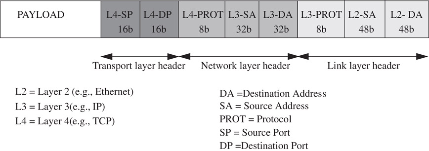
Figure 50.1This figure shows some of the header fields (and their widths) that might be used for classifying the packet. Although not shown in this figure, higher layer (e.g., application-level) headers may also be used.
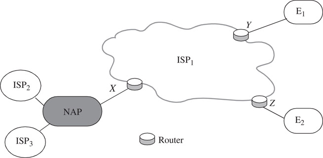
Figure 50.2Example network of an ISP (ISP1) connected to two enterprise networks (E1 and E2) and to two other ISP networks across a network access point (NAP).
Table 50.1Examples of Services Enabled by Packet Classification
|
Service |
Example |
|
Packet Filtering |
Deny all traffic from ISP3 (on interface X) destined to E2. |
|
Policy Routing |
Send all voice-over-IP traffic arriving from E1 (on interface Y) and destined to E2 via a separate ATM network. |
|
Accounting & Billing |
Treat all video traffic to E1 (via interface Y) as highest priority and perform accounting for the traffic sent this way. |
|
Traffic Rate Limiting |
Ensure that ISP2 does not inject more than 10 Mbps of email traffic and 50 Mbps of total traffic on interface X. |
|
Traffic Shaping |
Ensure that no more than 50 Mbps of web traffic is injected into ISP2 on interface X. |
Table 50.2 shows the flows that an incoming packet must be classified into by the router at interface X. Note that the flows specified may or may not be mutually exclusive. For example, the first and second flows in Table 50.2 overlap. This is common in practice, and when no explicit priorities are specified, we follow the convention that rules closer to the top of the list take priority (referred to as the “First matching rule in table” tie-breaker rule in Chapter 49).
Table 50.2Flows That an Incoming Packet Must be Classified Into by the Router at Interface X in Figure 50.2
|
Flow |
Relevant Packet Fields: |
|
Email and from ISP2 |
Source Link-layer Address, Source Transport port number |
|
From ISP2 |
Source Link-layer Address |
|
From ISP3 and going to E2 |
Source Link-layer Address, Destination Network-Layer Address |
|
All other packets |
– |
Each rule of a classifier has d components. R[i] is the ith component of rule R, and is a regular expression on the ith field of the packet header. A packet P is said to match rule R, if ∀i, the ith field of the header of P satisfies the regular expression R[i]. In practice, a rule component is not a general regular expression but is often limited by syntax to a simple address/mask or operator/number(s) specification. In an address/mask specification, a 0 (respectively 1) at bit position x in the mask denotes that the corresponding bit in the address is a don’t care (respectively significant) bit. Examples of operator/number(s) specifications are eq 1232 and range 34–9339. Note that a prefix can be specified as an address/mask pair where the mask is contiguous — i.e., all bits with value 1 appear to the left of bits with value 0 in the mask. It can also be specified as a range of width equal to 2t where t = 32 − prefixlength. Most commonly occurring specifications can be represented by ranges. An example real-life classifier in four dimensions is shown in Table 50.3. By convention, the first rule R1 is of highest priority and rule R7 is of lowest priority. Some example classification results are shown in Table 50.4.
Table 50.3An Example 4-Dimensional Real-Life Classifier
Table 50.4Example Classification Results from the Real-Life Classifier of Table 50.3
Longest prefix matching for routing lookups is a special-case of one-dimensional packet classification. All packets destined to the set of addresses described by a common prefix may be considered to be part of the same flow. The address of the next hop where the packet should be forwarded to is the associated action. The length of the prefix defines the priority of the rule.
50.2Performance Metrics for Classification Algorithms
1.Search speed—Faster links require faster classification. For example, links running at 10Gbps can bring 31.25 million packets per second (assuming minimum sized 40 byte TCP/IP packets).
2.Low storage requirements—Small storage requirements enable the use of fast memory technologies like SRAM (Static Random Access Memory). SRAM can be used as an on-chip cache by a software algorithm and as on-chip SRAM for a hardware algorithm.
3.Ability to handle large real-life classifiers.
4.Fast updates—As the classifier changes, the data structure needs to be updated. We can categorize data structures into those which can add or delete entries incrementally, and those which need to be reconstructed from scratch each time the classifier changes. When the data structure is reconstructed from scratch, we call it “pre-processing”. The update rate differs among different applications: a very low update rate may be sufficient in firewalls where entries are added manually or infrequently, whereas a router with per-flow queues may require very frequent updates.
5.Scalability in the number of header fields used for classification.
6.Flexibility in specification—A classification algorithm should support general rules, including prefixes, operators (range, less than, greater than, equal to, etc.) and wildcards. In some applications, non-contiguous masks may be required.
For the next few sections, we will use the example classifier in Table 50.5 repeatedly. The classifier has six rules in two fields labeled F1 and F2; each specification is a prefix of maximum length 3 bits. We will refer to the classifier as C = {Rj} and each rule Rj as a 2-tuple: .
Table 50.5Example 2-Dimensional Classifier
|
Rule |
F1 |
F2 |
|
R1 |
00* |
00* |
|
R2 |
0* |
01* |
|
R3 |
1* |
0* |
|
R4 |
00* |
0* |
|
R5 |
0* |
1* |
|
R6 |
* |
1* |
50.3.1.1Bounds from Computational Geometry
There is a simple geometric interpretation of packet classification. While a prefix represents a contiguous interval on the number line, a two-dimensional rule represents a rectangle in two-dimensional euclidean space, and a rule in d dimensions represents a d-dimensional hyper-rectangle. A classifier is therefore a collection of prioritized hyper-rectangles, and a packet header represents a point in d dimensions. For example, Figure 50.3 shows the classifier in Table 50.5 geometrically in which high priority rules overlay lower priority rules. Classifying a packet is equivalent to finding the highest priority rectangle that contains the point representing the packet. For example, point P(011,110) in Figure 3 would be classified by rule R5.
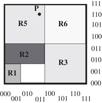
Figure 50.3Geometric representation of the classifier in Table 50.5. A packet represents a point, for instance P(011,110) in two-dimensional space. Note that R4 is hidden by R1 and R2.
There are several standard geometry problems such as ray shooting, point location and rectangle enclosure that resemble packet classification. Point location involves finding the enclosing region of a point, given a set of non-overlapping regions. The best bounds for point location in N rectangular regions and d > 3 dimensions are O(log N) time with O(Nd) space;* or O((log N)d−1) time with O(N) space [1,2]. In packet classification, hyper-rectangles can overlap, making classification at least as hard as point location. Hence, a solution is either impracticably large (with 100 rules and 4 fields, Nd space is about 100MBytes) or too slow ((log N)d−1 is about 350 memory accesses).
We can conclude that: (1) Multi-field classification is considerably more complex than one-dimensional longest prefix matching, and (2) Complexity may require that practical solutions use heuristics.
50.3.1.2Range Lookups
Packet classification is made yet more complex by the need to match on ranges as well as prefixes. The cases of looking up static arbitrary ranges, and dynamic conflict-free ranges in one dimension have been discussed in Chapter 49. One simple way to handle dynamic arbitrary (overlapping) ranges is to convert each W-bit range to a set of 2W − 2 prefixes (see Table 50.6) and then use any of the longest prefix matching algorithms detailed in Chapter 49, thus resulting in O(NW) prefixes for a set consisting of N ranges.
Table 50.6Example 4-Bit Ranges and Their Constituent Prefixes
|
Range |
Constituent Prefixes |
|
[4, 7] |
01** |
|
[3, 8] |
0011,01**,1000 |
|
[1, 14] |
0001,001*,01**,10**,110*,1110 |
50.3.2Taxonomy of Classification Algorithms
The classification algorithms we will describe here can be categorized into the four classes shown in Table 50.7.
Table 50.7Categories (not Non-overlapping) of Classification Algorithms
|
Category |
Algorithms |
|
Basicdatastructures |
Linear search, caching, hierarchical tries, set-pruning tries |
|
Geometry-based |
Grid-of-tries, AQT, FIS |
|
Heuristic |
RFC, hierarchical cuttings, tuple-space search |
|
Hardware |
Ternary CAM, bitmap-intersection (and variants) |
We now proceed to describe representative algorithms from each class.
50.3.3.1Linear Search
The simplest data structure is a linked-list of rules stored in order of decreasing priority. A packet is compared with each rule sequentially until a rule is found that matches all relevant fields. While simple and storage-efficient, this algorithm clearly has poor scaling properties; the time to classify a packet grows linearly with the number of rules.
50.3.3.2Hierarchical Tries
A d-dimensional hierarchical radix trie is a simple extension of the one dimensional radix trie data structure, and is constructed recursively as follows. If d is greater than 1, we first construct a 1-dimensional trie, called the F1-trie, on the set of prefixes {Rj1}, belonging to dimension F1 of all rules in the classifier, . For each prefix, p, in the F1-trie, we recursively construct a (d − 1)-dimensional hierarchical trie, Tp, on those rules which specify exactly p in dimension F1, i.e., on the set of rules {Rj : Rj1 = p}. Prefix p is linked to the trie Tp using a next-trie pointer. The storage complexity of the data structure for an N-rule classifier is O(NdW). The data structure for the classifier in Table 50.5 is shown in Figure 50.4. Hierarchical tries are sometimes called “multi-level tries,” “backtracking-search tries,” or “trie-of-tries”.
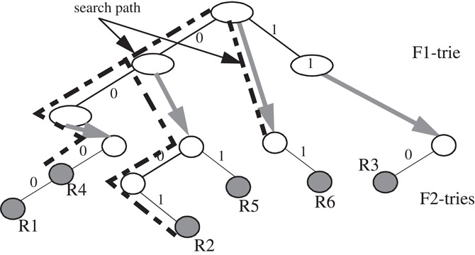
Figure 50.4A hierarchical trie data structure. The gray pointers are the “next-trie” pointers. The path traversed by the query algorithm on an incoming packet (000, 010) is shown.
Classification of an incoming packet (v1, v2, …, vd) proceeds as follows. The query algorithm first traverses the F1-trie based on the bits in v1. At each F1-trie node encountered, the algorithm follows the next-trie pointer (if present) and traverses the (d − 1)-dimensional trie. The query time complexity for d-dimensions is therefore O(Wd). Incremental updates can be carried out similarly in O(d2W) time since each component of the updated rule is stored in exactly one location at maximum depth O(dW).
50.3.3.3Set-Pruning Tries
A set-pruning trie data structure [3] is similar, but with reduced query time obtained by replicating rules to eliminate recursive traversals. The data structure for the classifier in Table 50.5 is shown in Figure 50.5. The query algorithm for an incoming packet (v1, v2, …, vd) need only traverse the F1-trie to find the longest matching prefix of v1, follow its next-trie pointer (if present), traverse the F2-trie to find the longest matching prefix of v1, and so on for all dimensions. The rules are replicated to ensure that every matching rule will be encountered in the path. The query time is reduced to O(dW) at the expense of increased storage of O(NddW) since a rule may need to be replicated O(Nd) times. Update complexity is O(Nd), and hence, this data structure works only for relatively static classifiers.
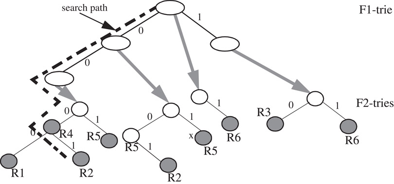
Figure 50.5A set-pruning trie data structure. The gray pointers are the “next-trie” pointers. The path traversed by the query algorithm on an incoming packet (000, 010) is shown.
50.3.4.1Grid-of-Tries
The grid-of-tries data structure, proposed by Srinivasan et al. [4] for 2-dimensional classification, reduces storage space by allocating a rule to only one trie node as in a hierarchical trie, and yet achieves O(W) query time by pre-computing and storing a switch pointer in some trie nodes. A switch pointer is labeled with “0’ or “1’ and guides the search process. The conditions which must simultaneously be satisfied for a switch pointer labeled b (b = ’0’ or “1’) to exist from a node w in the trie Tw to a node x of another trie Tx are (see Figure 50.6):
1.Tx and Tw are distinct tries built on the prefix components of dimension F2. Tx and Tw are pointed to by two distinct nodes, say r and s respectively of the same trie, T, built on prefix components of dimension F1.
2.The bit-string that denotes the path from the root node to node w in trie Tw concatenated with the bit b is identical to the bit-string that denotes the path from the root node to node x in the trie Tx.
3.Node w does not have a child pointer labeled b, and
4.Node s in trie T is the closest ancestor of node r that satisfies the above conditions.
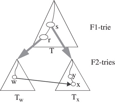
Figure 50.6The conditions under which a switch pointer exists from node w to node x.
If the query algorithm traverses paths U1(s, root(Tx), y, x) and U2(r, root(Tw), w) in a hierarchical trie, it need only traverse the path (s, r, root(Tw), w, x) on a grid-of-tries. This is because paths U1 and U2 are identical (by condition 2 above) till U1 terminates at node w because it has no child branch (by condition 3 above). The switch pointer eliminates the need for backtracking in a hierarchical trie without the storage overhead of a set-pruning trie. Each bit of the packet header is examined at most once, so the time complexity reduces to O(W), while storage complexity O(NW) is the same as a 2-dimensional hierarchical trie. However, the presence of switch pointers makes incremental updates difficult, so the authors recommend rebuilding the data structure (in time O(NW)) for each update. An example of the grid-of-tries data structure is shown in Figure 50.7.
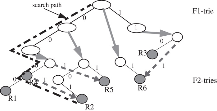
Figure 50.7The grid-of-tries data structure. The switch pointers are shown dashed. The path traversed by the query algorithm on an incoming packet (000, 010) is shown.
Reference 4 reports 2MBytes of storage for a 20,000 two-dimensional classifier with destination and source IP prefixes in a maximum of 9 memory accesses.
Grid-of-tries works well for two dimensional classification, and can be used for the last two dimensions of a multi-dimensional hierarchical trie, decreasing the classification time complexity by a factor of W to O(NWd−1). As with hierarchical and set-pruning tries, grid-of-tries handles range specifications by splitting into prefixes.
50.3.4.2Cross-Producting
Cross-producting [4] is suitable for an arbitrary number of dimensions. Packets are classified by composing the results of separate 1-dimensional range lookups for each dimension as explained below.
Constructing the data structure involves computing a set of ranges (basic intervals), Gk, of size sk = |Gk|, projected by rule specifications in each dimension k, 1 ≤ k ≤ d. Let , 1 ≤ j ≤ sk, denote the jth range in Gk. may be encoded simply as j in the kth dimension. A cross-product table CT of size is constructed, and the best matching rule for each entry , , 1 ≤ k ≤ d is pre-computed and stored. Classifying a packet (v1, v2, …, vd) involves a range lookup in each dimension k to identify the range containing point vk. The tuple (or, if using the above encoding for , the tuple < i1, i2, …, id > ) is then found in the cross-product table CT which contains the pre-computed best matching rule. Figure 50.8 shows an example.
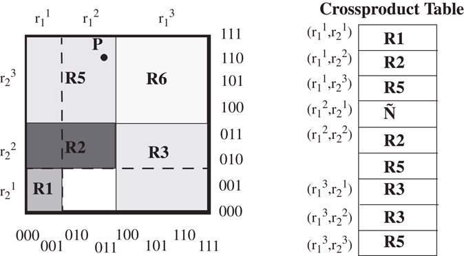
Figure 50.8The table produced by the crossproducting algorithm and its geometric representation.
Given that N prefixes lead to at most 2N − 2 ranges, sk ≤ 2N and CT is of size O(Nd). The lookup time is O(dtRL) where tRL is the time complexity of finding a range in one dimension. Because of its high worst case storage complexity, cross-producting is suitable only for very small classifiers. Reference [4] proposes using an on-demand cross-producting scheme together with caching for classifiers bigger than 50 rules in five dimensions. Updates require reconstruction of the cross-product table, and so cross-producting is suitable for relatively static classifiers.
50.3.4.3A 2-Dimensional Classification Scheme [5]
Lakshman and Stiliadis [5] propose a 2-dimensional classification algorithm where one dimension, say F1, is restricted to have prefix specifications while the second dimension, F2, is allowed to have arbitrary range specifications. The data structure first builds a trie on the prefixes of dimension F1, and then associates a set Gw of non-overlapping ranges to each trie node, w, that represents prefix p. These ranges are created by (possibly overlapping) projections on dimension F2 of those rules, Sw, that specify exactly p in dimension F1. A range lookup data structure (e.g., an array or a binary search tree) is then constructed on Gw and associated with trie node w. An example is shown in Figure 50.9.
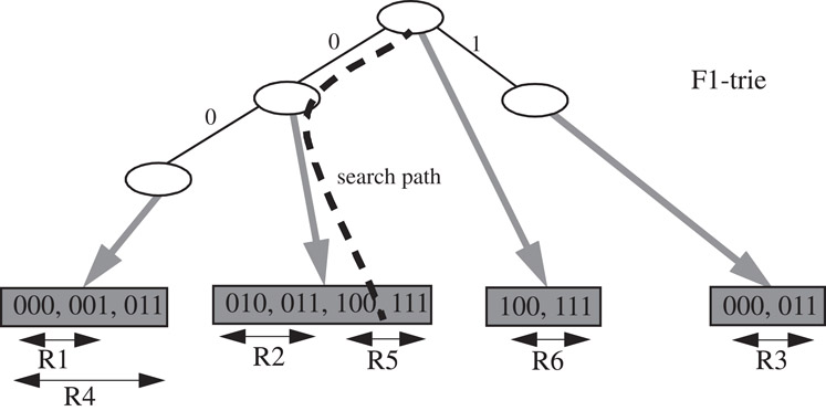
Figure 50.9The data structure of [5] for the example classifier of Table 50.5. The search path for example packet P(011, 110) resulting in R5 is also shown.
Searching for point P(v1, v2) involves a range lookup in data structure Gw for each trie node, w, encountered. The search in Gw returns the range containing v2, and hence the best matching rule. The highest priority rule is selected from the rules {Rw} for all trie nodes encountered during the traversal.
The storage complexity is O(NW) because each rule is stored only once in the data structure. Queries take O(W log N) time because an O(log N) range lookup is performed for every node encountered in the F1-trie. This can be reduced to O(W + log N) using fractional cascading [6], but that makes incremental updates impractical.
50.3.4.4Area-Based Quadtree
The Area-based Quadtree (AQT) was proposed by Buddhikot et al. [7] for two-dimensional classification. AQT allows incremental updates whose complexity can be traded off with query time by a tunable parameter. Each node of a quadtree [6] represents a two dimensional space that is decomposed into four equal sized quadrants, each of which is represented by a child node. The initial two dimensional space is recursively decomposed into four equal-sized quadrants till each quadrant has at most one rule in it (Figure 50.10 shows an example of the decomposition). Rules are allocated to each node as follows. A rule is said to cross a quadrant if it completely spans at least one dimension of the quadrant. For instance, rule R6 spans the quadrant represented by the root node in Figure 50.10, while R5 does not. If we divide the 2-dimensional space into four quadrants, rule R5 crosses the north-west quadrant while rule R3 crosses the south-west quadrant. We call the set of rules crossing the quadrant represented by a node in dimension k, the k-crossing filter set (k-CFS) of that node.
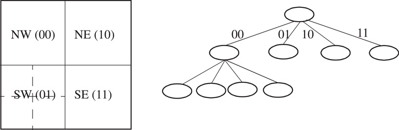
Figure 50.10A quadtree constructed by decomposition of two-dimensional space. Each decomposition results in four quadrants.
Two instances of the same data structure are associated with each quadtree node—each stores the rules in k-CFS (k = 1,2). Since rules in crossing filter sets span at least one dimension, only the range specified in the other dimension need be stored. Queries proceed two bits at a time by transposing one bit from each dimension, with two 1-dimensional lookups being performed (one for each dimension on k-CFS) at each node. Figure 50.11 shows an example.
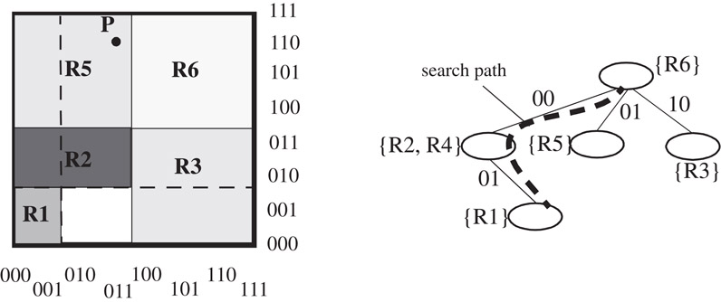
Figure 50.11An AQT data structure. The path traversed by the query algorithm on an incoming packet (000, 010) yields R1 as the best matching rule.
Reference 7 proposes an efficient update algorithm that, for N two-dimensional rules, has O(NW) space complexity, O(α W) search time and update time, where α is a tunable integer parameter.
50.3.4.5Fat Inverted Segment Tree (FIS-tree)
Feldman and Muthukrishnan [8] propose the Fat Inverted Segment tree (FIS-tree) for two dimensional classification as a modification of a segment tree. A segment tree [6] stores a set S of possibly overlapping line segments to answer queries such as finding the highest priority line segment containing a given point. A segment tree is a balanced binary search tree containing the end points of the line segments in S. Each node, w, represents a range Gw, the leaves represent the original line segments in S, and parent nodes represent the union of the ranges represented by their children. A line segment is allocated to a node w if it contains Gw but not Gparent(w). The highest priority line segment allocated to a node is pre-computed and stored at the node. A query traverses the segment tree from the root, calculating the highest priority of all the pre-computed segments encountered. Figure 50.12 shows an example segment tree.
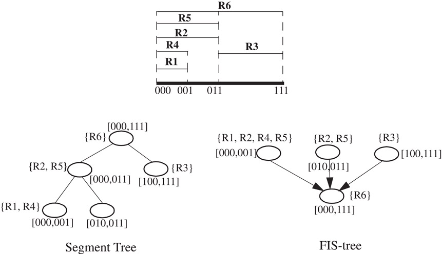
Figure 50.12The segment tree and the 2-level FIS-tree for the classifier of Table 50.5.
An FIS-tree is a segment tree with two modifications: (1) The segment tree is compressed (made “fat” by increasing the degree to more than two) in order to decrease its depth and occupies a given number of levels l, and (2) Up-pointers from child to parent nodes are used. The data structure for 2-dimensions consists of an FIS-tree on dimension F1 and a range lookup data associated with each node. An instance of the range lookup data structure associated with node w of the FIS-tree stores the ranges formed by the F2-projections of those classifier rules whose F1-projections were allocated to w.
A query for point P(v1, v2) first solves the range lookup problem on dimension F1. This returns a leaf node of the FIS-tree representing the range containing the point v1. The query algorithm then follows the up-pointers from this leaf node towards the root node, carrying out 1-dimensional range lookups at each node. The highest priority rule containing the given point is calculated at the end of the traversal.
Queries on an l-level FIS-tree have complexity O((l + 1)tRL) with storage complexity O(ln1+1/l), where tRL is the time for a 1-dimensional range lookup. Storage space can be traded off with search time by varying l. Modifications to the FIS-tree are necessary to support incremental updates—even then, it is easier to support inserts than deletes [8]. The static FIS-tree can be extended to multiple dimensions by building hierarchical FIS-trees, but the bounds are similar to other methods studied earlier [8].
Measurements on real-life 2-dimensional classifiers are reported in Reference 8 using the static FIS-tree data structure. Queries took 15 or fewer memory operations with a two level tree, 4–60 K rules and 5 MBytes of storage. Large classifiers with one million 2-dimensional rules required 3 levels, 18 memory accesses per query and 100MBytes of storage.
50.3.4.6Dynamic Multi-Level Tree Algorithms
Two algorithms, called Heap-on-Trie (HoT) and Binarysearchtree-on-Trie (BoT) are introduced in Reference 9 that build a heap and binary search tree respectively on the last dimension, and multi-level tries on all the remaining d − 1 dimensions. If W = O(log N): HoT has query complexity O(logdN), storage complexity O(N logdN), and update complexity O(logd+1N); and BoT has query complexity O(logd+1N), storage complexity O(N logdN), and update complexity O(logdN). If W ≠ O(log N), each of the above complexity formulae need to be modified to replace a factor O(logd−1N) with O(Wd−1).
As we saw in Section 50.3.1.1, the packet classification problem is expensive to solve in the worst-case—theoretical bounds state that solutions to multi-field classification either require storage that is geometric, or a number of memory accesses that is polylogarithmic, in the number of classification rules. We can expect that classifiers in real networks have considerable structure and redundancy that might be exploited by a heuristic. That is the motivation behind the algorithms described in this section.
50.3.5.1Recursive Flow Classification (RFC)
RFC [10] is a heuristic for packet classification on multiple fields. Classifying a packet involves mapping S bits in the packet header to a T bit action identifier, where T = log N, T≪S. A simple, but impractical method could pre-compute the action for each of the 2S different packet headers, yielding the action in one step. RFC attempts to perform the same mapping over several phases, as shown in Figure 50.13; at each stage the algorithm maps one set of values to a smaller set. In each phase a set of memories return a value shorter (i.e., expressed in fewer bits) than the index of the memory access. The algorithm, illustrated in Figure 50.14, operates as follows:
1.In the first phase, d fields of the packet header are split up into multiple chunks that are used to index into multiple memories in parallel. The contents of each memory are chosen so that the result of the lookup is narrower than the index.
2.In subsequent phases, memories are indexed using the results from earlier phases.
3.In the final phase, the memory yields the action.
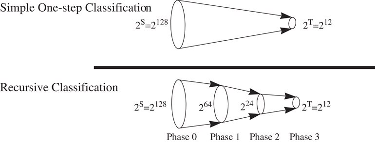
Figure 50.13Showing the basic idea of Recursive Flow Classification. The reduction is carried out in multiple phases, with a reduction in phase I being carried out recursively on the image of the phase I − 1. The example shows the mapping of 2S bits to 2T bits in three phases.
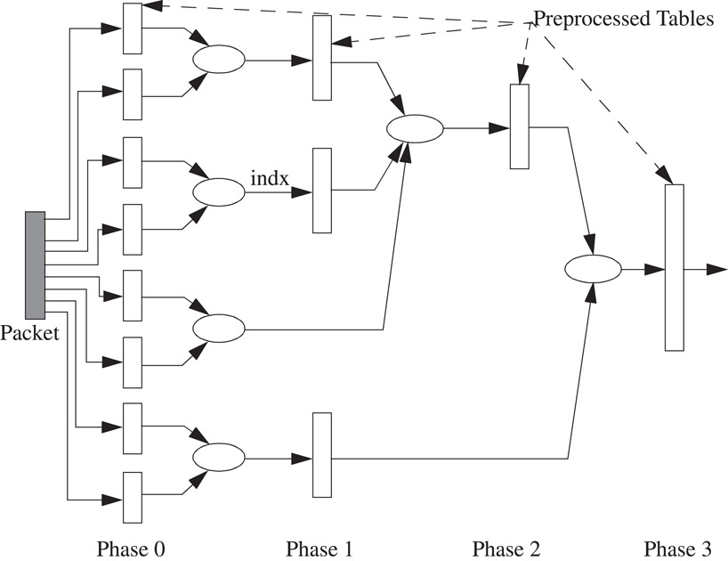
Figure 50.14Packet flow in RFC.
The algorithm requires construction of the contents of each memory detailed in Reference 10. This paper reports that with real-life four-dimensional classifiers of up to 1700 rules, RFC appears practical for 10Gbps line rates in hardware and 2.5Gbps rates in software. However, the storage space and pre-processing time grow rapidly for classifiers larger than 6000 rules. An optimization described in Reference 10 reduces the storage requirement of a 15,000 four-field classifier to below 4MBytes.
50.3.5.2Hierarchical Intelligent Cuttings (HiCuts)
HiCuts [11] partitions the multi-dimensional search space guided by heuristics that exploit the structure of the classifier. Each query leads to a leaf node in the HiCuts tree, which stores a small number of rules that can be searched sequentially to find the best match. The characteristics of the decision tree (its depth, degree of each node, and the local search decision to be made at each node) are chosen while pre-processing the classifier based on its characteristics (see Reference 11 for the heuristics used).
Each node, v, of the tree represents a portion of the geometric search space. The root node represents the complete d-dimensional space, which is partitioned into smaller geometric sub-spaces, represented by its child nodes, by cutting across one of the d dimensions. Each sub-space is recursively partitioned until no sub-space has more than B rules, where B is a tunable parameter of the pre-processing algorithm. An example is shown in Figure 50.15 for two dimensions with B = 2.
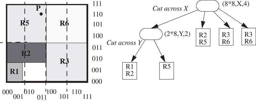
Figure 50.15A possible HiCuts tree for the example classifier in Table 50.5. Each ellipse in the tree denotes an internal node v with a tuple <size of 2-dimensional space represented, dimension to cut across, number of children>. Each square is a leaf node which contains the actual classifier rules.
Parameters of the HiCuts algorithm can be tuned to trade- off query time against storage requirements. On 40 real-life four-dimensional classifiers with up to 1,700 rules, HiCuts requires less than 1 MByte of storage with a worst case query time of 20 memory accesses, and supports fast updates.
50.3.5.3Tuple Space Search
The basic tuple space search algorithm [12] decomposes a classification query into a number of exact match queries. The algorithm first maps each d-dimensional rule into a d-tuple whose ith component stores the length of the prefix specified in the ith dimension of the rule (the scheme supports only prefix specifications). Hence, the set of rules mapped to the same tuple are of a fixed and known length, and can be stored in a hash table. Queries perform exact match operations on each of the hash tables corresponding to all possible tuples in the classifier. An example is shown in Figure 50.16.
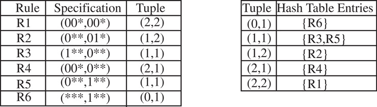
Figure 50.16The tuples and associated hash tables in the tuple space search scheme for the example classifier of Table 50.5.
Query time is M hashed memory accesses, where M is the number of tuples in the classifier. Storage complexity is O(N) since each rule is stored in exactly one hash table. Incremental updates are supported and require just one hashed memory access to the hashed table associated with the tuple of the modified rule. In summary, the tuple space search algorithm performs well for multiple dimensions in the average case if the number of tuples is small. However, the use of hashing makes the time complexity of searches and updates non-deterministic. The number of tuples could be very large, up to O(Wd), in the worst case. Furthermore, since the scheme supports only prefixes, the storage complexity increases by a factor of O(Wd) for generic rules as each range could be split into W prefixes in the manner explained in Section 50.3.1. Of course, the algorithm becomes attractive for real-life classifiers that have a small number of tuples.
50.3.6Hardware-Based Algorithms
50.3.6.1Ternary CAMs
A TCAM stores each W-bit field as a (val, mask) pair; where val and mask are each W-bit numbers. A mask of “0’ wildcards the corresponding bit position. For example, if W = 5, a prefix 10* will be stored as the pair (10000, 11000). An element matches a given input key by checking if those bits of val for which the mask bit is “1’, match those in the key.
A TCAM is used as shown in Figure 50.17. The TCAM memory array stores rules in decreasing order of priorities, and compares an input key against every element in the array in parallel. The N-bit bit-vector, matched, indicates which rules match and so the N-bit priority encoder indicates the address of the highest priority match. The address is used to index into a RAM to find the action associated with this prefix. TCAMs are being increasingly deployed because of their simplicity of use and speed (as they are able to do classification in hardware at the rate of the hardware clock).
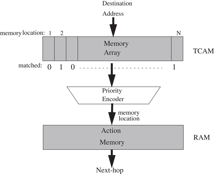
Figure 50.17The classification operation using a ternary CAM. The packet header in this example is assumed to comprise only the destination address.
Several companies today ship 9Mb TCAMs capable of single and multi-field classification in as little as 10 ns. Both faster and denser TCAMs can be expected in the near future. There are, however, some disadvantages to TCAMs:
1.A TCAM is less dense than a RAM, storing fewer bits in the same chip area. One bit in an SRAM typically requires 4–6 transistors, while one bit in a TCAM requires 11–15 transistors [13]. A 9Mb TCAM running at 100 MHz costs about $200 today, while the same amount of SRAM costs less than $10. Furthermore, range specifications need to be split into multiple masks, reducing the number of entries by up to (2W − 2)d in the worst case. If only two 16-bit dimensions specify ranges, this is a multiplicative factor of 900. Newer TCAMs, based on DRAM technology, have been proposed and promise higher densities.
2.TCAMs dissipate more power than RAM solutions because an address is compared against every TCAM element in parallel. At the time of writing, a 9Mb TCAM chip running at 100 MHz dissipates about 10–15 watts (the exact number varies with manufacturer). In contrast, a similar amount of SRAM running at the same speed dissipates 1W.
3.A TCAM is more unreliable while being in operational use in a router in the field than a RAM, because a soft-error (error caused by alpha particles and package impurities that can flip a bit of memory from 0 to 1, or vice-versa) could go undetected for a long amount of time. In a SRAM, only one location is accessed at any time, thus enabling easy on-the-fly error detection and correction. In a TCAM, wrong results could be given out during the time that the error is undetected – which is particularly problematic in such applications as filtering or security.
However, the above disadvantages of a TCAM need to be weighed against its enormous simplicity of use in a hardware platform. Besides, it is the only known “algorithm” that is capable of doing classification at high speeds without explosion in either storage space or time.
Due to their high cost and power dissipation, TCAMs will probably remain unsuitable in the near future for (1) Large classifiers (512K-1M rules) used for microflow recognition at the edge of the network, (2) Large classifiers (256-512 K rules) used at edge routers that manage thousands of subscribers (with a few rules per subscriber). Of course, software-based routers need to look somewhere else.
50.3.6.2Bitmap-Intersection
The bitmap-intersection classification scheme, proposed in Reference 5, is based on the observation that the set of rules, S, that match a packet is the intersection of d sets, Si, where Si is the set of rules that match the packet in the ith dimension alone. While cross-producting pre-computes S and stores the best matching rule in S, this scheme computes S and the best matching rule during each classification operation.
In order to compute intersection of sets in hardware, each set is encoded as an N-bit bitmap where each bit corresponds to a rule. The set of matching rules is the set of rules whose corresponding bits are “1’ in the bitmap. A query is similar to cross-producting: First, a range lookup is performed in each of the d dimensions. Each lookup returns a bitmap representing the matching rules (pre-computed for each range) in that dimension. The d sets are intersected (a simple bit-wise AND operation) to give the set of matching rules, from which the best matching rule is found. See Figure 50.18 for an example.
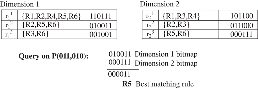
Figure 50.18Bitmap tables used in the “bitmap-intersection” classification scheme. See Figure 50.8 for a description of the ranges. Also shown is classification query on an example packet P(011, 110).
Since each bitmap is N bits wide, and there are O(N) ranges in each of d dimensions, the storage space consumed is O(dN2). Query time is O(dtRL + dN/w) where tRL is the time to do one range lookup and w is the memory width. Time complexity can be reduced by a factor of d by looking up each dimension independently in parallel. Incremental updates are not supported.
Reference [5] reports that the scheme can support up to 512 rules with a 33 MHz field-programmable gate array and five 1Mbit SRAMs, classifying 1Mpps. The scheme works well for a small number of rules in multiple dimensions, but suffers from a quadratic increase in storage space and linear increase in classification time with the size of the classifier. A variation is described in Reference 5 that decreases storage at the expense of increased query time. This work has been extended significantly by [14] by aggregating bitmaps wherever possible and thus decreasing the time spent in reading the bitmaps. Though the bitmap-intersection scheme is primarily meant for hardware, it is easy to see how it can be used in software, where the aggregated bitmap technique of [14] could be especially useful.
Please see Table 50.8 for a summary of the complexities of classification algorithms described in this chapter.
Table 50.8Complexity of Various Classification Algorithms
|
Algorithm |
Worst-Case Time Complexity |
Worst-Case Storage Complexity |
|
Linear Search |
N |
N |
|
Ternary CAM1 |
1 |
N |
|
Hierarchical Tries |
Wd |
NdW |
|
Set-pruning Tries |
dW |
Nd |
|
Grid-of-Tries |
Wd−1 |
NdW |
|
Cross-producting |
dW |
Nd |
|
FIS-tree |
(l + 1)W |
l * N1+1/l |
|
RFC |
d |
Nd |
|
Bitmap-intersection |
dW + N/memwidth |
dN2 |
|
HiCuts |
d |
Nd |
|
Tuple Space Search |
N |
N |
Note: N is the Number of Rules in d, W-bit Wide, Dimensions
1.M.H. Overmars and A.F. van der Stappen. “Range Searching and Point Location Among Fat Objects,” Journal of Algorithms, vol. 21, no. 3, pages 629–656, November 1996.
2.F. Preparata and M. I. Shamos. Computational Geometry: An Introduction, Springer-Verlag, 1985.
3.P. Tsuchiya. “A Search Algorithm for Table Entries with Non-Contiguous Wildcarding,” unpublished report, Bellcore.
4.V. Srinivasan, S. Suri, G. Varghese, and M. Waldvogel. “Fast and Scalable Layer four Switching,” Proceedings of ACM Sigcomm, pages 203–14, September 1998.
5.T.V. Lakshman and D. Stiliadis. “High-Speed Policy-based Packet Forwarding Using Efficient Multi-dimensional Range Matching”, Proceedings of ACM Sigcomm, pages 191–202, September 1998.
6.M. de Berg, M. van Kreveld, and M. Overmars. Computational Geometry: Algorithms and Applications, Springer-Verlag, 2nd rev. ed. 2000.
7.M.M. Buddhikot, S. Suri, and M. Waldvogel. “Space Decomposition Techniques for Fast Layer-4 Switching,” Proceedings of Conference on Protocols for High Speed Networks, pages 25–41, August 1999.
8.A. Feldman and S. Muthukrishnan. “Radeoffs for Packet Classification,” Proceedings of Infocom, vol. 3, pages 1193–202, March 2000.
9.P. Gupta and N. McKeown. “Dynamic Algorithms with Worst-case Performance for Packet Classification,” Proc. IFIP Networking, pages 528–39, May 2000, Paris, France.
10.P. Gupta and N. McKeown. “Packet Classification on Multiple Fields,” Proc. Sigcomm, Computer Communication Review, vol. 29, no. 4, pp 147–60, September 1999, Harvard University.
11.P. Gupta and N. McKeown. “Packet Classification using Hierarchical Intelligent Cuttings,” Proc. Hot Interconnects VII, August 99, Stanford. This paper is also available in IEEE Micro, pages 34–41, vol. 20, no. 1, January/February 2000.
12.V. Srinivasan, S. Suri, and G. Varghese. “Packet Classification using Tuple Space Search,” Proceedings of ACM Sigcomm, pages 135–46, September 1999.
13.F. Shafai, K.J. Schultz, G.F. R. Gibson, A.G. Bluschke and D.E. Somppi. “Fully Parallel 30-Mhz, 2.5 Mb CAM,” IEEE Journal of Solid-State Circuits, vol. 33, no. 11, November 1998.
14.F. Baboescu and G. Varghese. “Scalable Packet Classification,” Proc. Sigcomm, 2001.
*This chapter has been reprinted from first edition of this Handbook, without any content updates.
†We have used this author’s affiliation from the first edition of this handbook, but note that this may have changed since then.
‡A network access point is a network site which acts as an exchange point for Internet traffic. ISPs connect to the NAP to exchange traffic with other ISPs.
*The time bound for d ≤ 3 is O(log log N) [1] but has large constant factors.