
Dinesh P. Mehta
Colorado School of Mines
53.3Layout Data Structures: An Overview
Point Finding•Tile Insertion•Storage Requirements of the Corner Stitching Data Structure
53.5Corner Stitching Extensions
Expanded Rectangles•Trapezoidal Tiles•Curved Tiles•L-Shaped Tiles
Bisector List Quad Trees•k-d Trees• Multiple Storage Quad Trees• Quad List Quad Trees• Bounded Quad Trees• HV Trees• Hinted Quad Trees
VLSI (Very Large Scale Integration) is a technology that has enabled the manufacture of large circuits in silicon. It is not uncommon to have circuits containing millions of transistors, and this quantity continues to increase very rapidly. Designing a VLSI circuit is itself a very complex task and has spawned the area of VLSI design automation. The purpose of VLSI design automation is to develop software that is used to design VLSI circuits. The VLSI design process is sufficiently complex that it consists of the four steps shown in Figure 53.1. Architectural design is carried out by expert human engineers with some assistance from tools such as simulators. Logic design is concerned with the boolean logic required to implement a circuit. Physical design is concerned with the implementation of logic on a three dimensional physical structure: the VLSI chip. VLSI physical design consists of steps such as floorplanning, partitioning, placement, routing, circuit extraction, etc. Details about VLSI physical design automation may be found in References 1–3. Chapter 54 describes the rich area of data structures for floorplanning. In this chapter, our concern will be with the representation of a circuit in its “physical” form. In order to proceed with this endeavor, it is necessary to first understand the basics of VLSI technology.
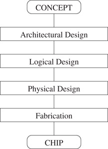
Figure 53.1The VLSI design stages.
We begin with the caveat that our presentation here only seeks to convey the basics of VLSI technology. Detailed knowledge about this area may be obtained from texts such as [4]. The transistor is the fundamental device in VLSI technology and may be viewed as a switch. It consists of a gate, a source, and a drain. The voltage on the gate controls the passage of current between the source and the drain. Thus, the gate can be used to switch the transistor “on” (current flows between the source and the drain) and “off” (no current flows). Basic logic elements such as the inverter (the NOT gate), the NAND gate, and the NOR gate are built using transistors. Transistors and logic gates can be manufactured in layers on a silicon disk called a wafer. Pure silicon is a semiconductor whose electrical resistance is between that of a conductor and an insulator. Its conductivity can be significantly improved by introducing “impurities” called dopants. N-type dopants such as phosphorus supply free electrons, while p-type dopants like boron supply holes. Dopants are diffused into the silicon wafer. This layer of the chip is called the diffusion layer and is further classified into n-type and p-type depending on the type of dopant used. The source and drain of a transistor are formed by separating two n-type regions with a p-type region (or vice versa). A gate is formed by sandwiching a silicon dioxide (an insulator) layer between the p-type region and a layer of polycrystalline silicon (a conductor). Figure 53.2 illustrates these concepts. Since polycrystalline silicon (poly) is a conductor, it is also used for short interconnections (wires). Up to this point, we have described the two layers (diff and poly) that are used to make all electronic devices. Although poly conducts electricity, it is not sufficient to complete all the interconnections using one layer. Modern chips usually have several layers of aluminum (“metal”), a conductor, separated from each other by insulators on top of the poly layer. These make it possible for the gates to be interconnected as specified in the design. Note that a layer of material X (e.g., poly) does not mean that there is a monolithic slab of poly over the entire chip area. The poly is only deposited where gates or wires are needed. The remaining areas are filled with insulating materials and for our purposes may be viewed as being empty. In addition to the layers as described above, it is necessary to have a mechanism for signals to pass between layers. This is achieved by contacts (to connect poly with diffusion or metal) and vias (to connect metal on different layers). Figure 53.3 shows the layout and a schematic of an nMOS inverter. We briefly describe the functioning of the inverter. If the input gate voltage is “0,” the transistor is switched off and there is no connection between the ground signal and the output. The voltage at the output is identical to that of the power source, which is a “1.” If the gate is at “1,” the transistor is switched on and there is a connection between the ground signal “0” and the output, making the output “0.”
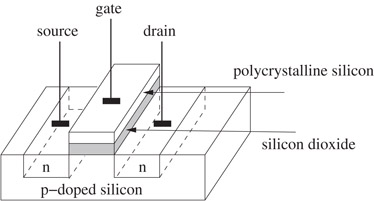
Figure 53.2A transistor.
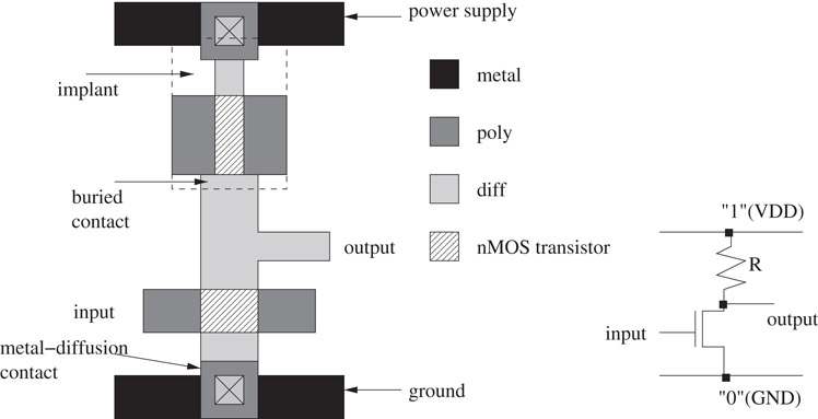
Figure 53.3An inverter.
The purpose of a layout data structure is to store and manipulate the rectangles on each layer. Some important high-level operations that a layout data structure must support are design-rule checking, layout compaction, and parasitic extraction.
Design Rule Checking (DRC): Design rules are the interface between the circuit designer and the process engineer. They specify geometric constraints on the layout so that the patterns on the processed wafer preserve the topology of the designs. An example of a design rule is that the width of a wire must be greater than a specified minimum. If this constraint is violated, it is possible that for the wire to be discontinuous because of errors in the fabrication process. Similarly, if two wires are placed too close to each other, they could touch each other. The DRC step verifies that all design rules have been met. Additional design rules for CMOS technology may be found in Reference 4, page 142.
Parasitic Extraction: Each layer of the chip has a resistance and a capacitance that are critical to the estimation of circuit performance. Inductance is usually less important on the chip, but has greater impact on the I/O components of the chip. Capacitance, resistance, and inductance are commonly referred to as “parasitics.” After a layout has been created, the parasitics must be computed in order to verify that the circuit will meet its performance goals. (Performance is usually measured by clock cycle times and power dissipation.) The parasitics are computed from the geometry of the layout. For example, the resistance of a rectangular slab of metal is , where ρ is the resistivity of the metal and l, w, and t are the slab’s length, width, and thickness, respectively. See [4, Chapter 4] for more examples.
Compaction: The compaction step, as its name suggests, tries to make the layout as small as possible without violating any design rules. This reduces the area of the chip, which could result in more chips being manufactured from a single wafer, which significantly reduces cost per chip. Interestingly, the cost of a chip could grow as a power of five of its area [5] making it imperative that area be minimized! Two-dimensional compaction is NP-hard, but one-dimensional compaction can be carried out in polynomial time. Heuristics for 2D compaction often iteratively interleave one-dimensional compactions in the x- and y-directions. For more details, see [6].
53.3Layout Data Structures: An Overview
There are two types of layout data structures that are based on differing philosophies. The first is in the context of a layout editor. Here, the idea is that a user manually designs the layout, for example, by inserting rectangles of the appropriate dimensions at the appropriate layer. This customized approach is used for library cells. The MAGIC system [7] developed at U.C. Berkeley is an example of of a system that included a layout editor. MAGIC was in the public domain and was used to support classes on VLSI design in many universities. The layout editor context is especially important here because it permitted the developers of MAGIC to assume locality of reference; that is, a user is likely to perform several editing operations in the same area of the layout over a short period of time. The second philosophy is that the layout process is completely automated. This has the advantage that some user-interaction operations do not need to be supported and run time is critical. This approach is more common in industrial software, where automatic translation techniques convert electronic circuits into physical layouts. This philosophy is supported by the quad-tree and variants that were designed specifically for VLSI layout.
The corner stitching data structure was proposed by Ousterhout [8] to store non-overlapping rectilinear circuit components in MAGIC. The data structure is obtained by partitioning the layout area into horizontally maximal rectangular tiles. There are two types of tiles: solid and vacant, both of which are explicitly stored in the corner-stitching data structure. Tiles are obtained by extending horizontal lines from corners of all solid tiles until another solid tile or a boundary of the layout region is encountered. The set of solid and vacant tiles so obtained is unique for a given input. The partitioning scheme ensures that no two vacant or solid tiles share a vertical side. Each tile T is stored as a node which contains the coordinates of its bottom left corner, x1 and y1, and four pointers N, E, W, and S. N (respectively, E, W, S) points to the rightmost (respectively, topmost, bottommost, leftmost) tile neighboring its north (respectively, east, west, south) boundary. The x and y coordinates of the top right corner of T are and , respectively, and are easily obtained in O(1) time. Figure 53.4 illustrates the corner stitching data structure.
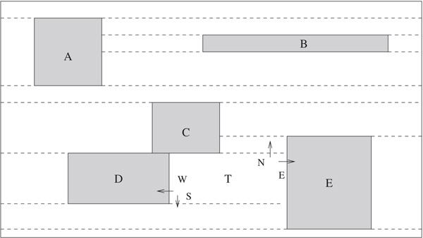
Figure 53.4The corner stitching data structure. Pointers (stitches) are shown for tile T.
The corner stitching data structure supports a rich set of operations.
1.Point Finding: given a tile T and a point p(x, y), search for the tile containing p by following a sequence of stitches starting at T.
2.Neighbor Finding: find all solid and vacant tiles that abut a given tile T.
3.Area Searches: determine whether any solid tiles intersect a given rectangular area R. This operation is used to determine whether a new solid tile can subsequently be inserted into area R. (Recall that tiles in a layer are not permitted to overlap.)
4.Directed Area Enumeration: enumerate all the tiles contained in a given rectangular area in a specified order. This is used during the compaction operation which may require tiles to be visited and compacted in a left-to-right order.
5.Tile Creation: insert a solid tile T into the data structure at a specified location.
6.Tile Deletion: delete a specified solid tile T from the data structure.
7.Plowing: translate a large piece of a design. Move other pieces of the design that lie in its path in the same direction.
8.Compaction: this refers to one-dimensional compaction.
We describe two operations to illustrate corner stitching.
Next, we focus on the point find operation because of its effect on the performance of corner stitching. The algorithm is presented below. Given a pointer to an arbitrary tile T in the layout, the algorithm seeks the tile in the layout containing the point P.
Tile Point_Find (Tile T, Point P) 1. begin 2. current = T; 3. while (P is not contained in current) 4. begin 5. while (P.y does not lie in current’s y-range) 6. if (P.y is above current) current = current; 7. else current = current; 8. while (P.x does not lie in current’s x-range) 9. if (P.x is to the right of current) current = current; 10. else current = current; 11. end 12. return (current); 13. end
Figure 53.5 illustrates the execution of the point find operation on a pathological example. From the start tile T, the while loop of line 5 follows north pointers until tile A is reached. We change directions at tile A since its y-range contains P. Next, west pointers are followed until tile F is reached (whose x-range contains P). Notice that the sequence of west moves causes the algorithm to descend in the layout resulting in a vertical position that is similar to that of the start tile! As a result of this misalignment, the outer while loop of the algorithm must execute repeatedly until the point is found (note that the point will eventually be found since the point find algorithm is guaranteed to converge).
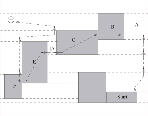
Figure 53.5Illustration of point find operation and misalignment.
This operation creates a new solid tile and inserts it into the layout. It accomplishes this by a sequence of split and merge operations. The split operation breaks a tile into two tiles along either a vertical or a horizontal line. The merge operation combines two tiles to form a rectangular tile. Algorithm Insert discusses the insertion of a rectangle into the layout.
Insert(A) // (x1, y1) and (x2, y2) are the bottom left and top right corners of A.
1.if (!AreaSearch(A)) return; //area is not empty, abort.
2.Let i = 0; Split Qi, the tile containing the north edge of A into two tiles along the line y = y2; Let T be the upper tile and Qi be the lower tile.
3.while (Qi does not contain the south edge of A)
a.Split Qi vertically into three tiles along x = x1 and x = x2; let the resulting tiles from left to right be Li, Qi, and Ri.
b.if (i > 0)
i.Merge Ri−1 and Li−1 into Ri and Li, respectively, if possible.
ii.Merge Qi−1 into Qi;
c.Let Qi+1 be the tile beneath Qi.
d.Increment i;
4.Split Qi along y = y1; Let Qi be the tile above the split and B the tile below the split; Split Qi into Li, Qi, and Ri using the lines x = x1 and x = x2;
5.Merge Qi and Qi−1 to get Qi. Qi is the newly inserted solid tile;
6.Merge Ri−1, Li−1 with neighboring tiles; if Ri (Li) gets merged, the merged tile is called Ri (Li). Merge Ri and Li with neighboring tiles;
Figure 53.6 shows the various steps involved in the insertion algorithm.
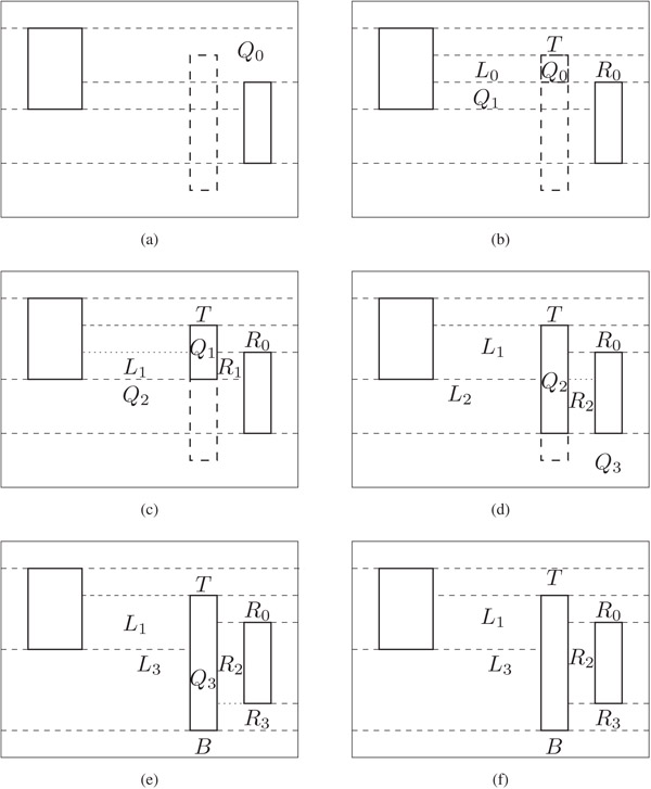
Figure 53.6Illustration of insertion.
The rectangle A to be inserted is represented by thick, dashed lines in Figure 53.6a. The coordinates of the bottom left and top right corners of A are (x1, y1) and (x2, y2), respectively. First, Step 1 of the algorithm uses AreaSearch to ensure that no solid tiles intersect A. Step 2 identifies tile Q0 as the vacant tile containing A’s north edge and splits it by the horizontal line y = y2 into two tiles: T above the split-line and Q0 below the split-line. Next, in the while loop of Step 3, Q0 is split by vertical lines at x1 and x2 to form L0, Q0, R0. Tile Q1 is the vacant tile below Q0. The resulting configuration is shown in Figure 53.6b. In the next iteration, Q1 is split to form L1, Q1, and R1. L0 merges into L1 and Q0 merges into Q1. Tile Q2 is the vacant tile below Q1. The resulting configuration is shown in Figure 53.6c. Next, Q2 is split to form L2, Q2, and R2. R1 is merged into R2 and Q1 merged into Q2. Figure 53.6d shows the configuration after Tile Q2 is processed. The vacant tile Q3 below Q2 contains R’s bottom edge and the while loop of Step 3 is exited. Steps 4, 5, and 6 of the algorithm result in the configuration of Figure 53.6e. The final layout is shown in Figure 53.6f.
53.4.3Storage Requirements of the Corner Stitching Data Structure
Unlike simpler data structures such as arrays and linked lists, it is not trivial to manually estimate the storage requirements of a corner stitched layout. For example, if n items are inserted into a linked list, then the amount of storage required is n multiplied by the number of bytes required by a single list node. Because of vacant tiles, the total number of nodes in corner stitching is considerably more than n and depends on the relative positions of the n rectangles. In References 9 and 10, a general formula for the memory requirements of the corner stitching data structure on a given layout. This formula requires knowledge about certain geometric properties of the layout called violations of the CV property and states that a corner stitching data structure representing a set of N solid, rectangular tiles with k violations contains 3N + 1 − k vacant tiles. Since each rectangular tile requires 28 bytes, the memory requirements are 28(4N + 1 − k) bytes.
53.5Corner Stitching Extensions
Expanded rectangles [11] expands solid tiles in the corner stitching data structure so that each tile contains solid material and the empty space around it. No extra tiles are needed to represent empty space. Thus, there are fewer tiles than in corner stitching. However, each tile now requires 44 rather than 28 bytes because additional fields are needed to store the coordinates of the solid portion of the tile. It was determined that expanded rectangles required less memory than corner stitching when the ratio of vacant to solid tiles in corner stitching was greater than 0.414. Operations on the expanded rectangles data structure are similar to those in corner stitching.
Marple et al. [12] developed a layout system called “Tailor” that was similar to MAGIC except that it allowed 45° layout. Thus, rectangular tiles were replaced by trapezoidal tiles. There are 9 types of trapezoidal tiles as shown in Figure 53.7. An additional field that stores the type of trapezoidal tile is used. The operations on Tailor are similar to those in MAGIC and are implemented in a similar way. It is possible to extend these techniques to arbitrary angles making it possible to describe arbitrary polygonal shapes.

Figure 53.7The different types of trapezoidal tiles.
Séquin and Façanha [13] proposed two generalizations to geometries including circles and arbitrary curved shapes, which arise in microelectromechanical systems (MEMS). As with its corner stitching-based predecessors, the layout area is decomposed in a horizontally maximal fashion into tiles. Consequently, tiles have upper and lower horizontal sides. Their left and right sides are represented by parameterized cubic Bezier curves or by composite paths composed of linear, circular, and spline segments. Strategies for reducing storage by minimizing the number of tiles and curve-sharing among tiles are discussed.
Mehta and Blust [14] extended Ousterhout’s corner stitching data structure to directly represent L- and other simple rectilinear shapes without partitioning them into rectangles. This results in a data structure that is topologically different from the other versions of corner stitching described above. A key property of this L-shaped corner stitching (LCS) data structure is that
1.All vacant tiles are either rectangles or L-shapes.
2.No two vacant tiles in the layout can be merged to form a vacant rectangle or L-shaped tile.
Figure 53.8 shows three possible configurations for the same set of solid tiles.
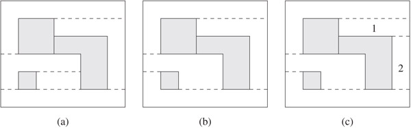
Figure 53.8Layouts represented by the L-shaped corner stitching data structure: Layout (c) is invalid because the vacant tiles 1 and 2 can be merged to form an L-shaped tile. Layouts (b) and (c) are both valid, illustrating that unlike RCS, the LCS data structure does not give a unique partition for a given set of solid tiles.
There are four L-shape types (Figure 53.9), one for each orientation of the L-shape. The L-shapes are numbered according to the quadrant represented by the two lines meeting at the single concave corner of the L-shape. Figure 53.10 describes the contents of L-shapes and rectangles in LCS and rectangles in the original rectangular corner stitching (RCS) data structure. The actual memory requirements of a node in bytes (last column of the table) are obtained by assuming that pointers and coordinates, each, require 4 bytes of storage, and by placing all the remaining bits into a single 4-byte word. Note that the space required by any L-shape is less than the space required by two rectangles in RCS and that the space required by a rectangle in LCS is equal to the space required by a rectangle in RCS. The following theorem has been proved in Reference 9:
Theorem 53.1
The LCS data structure never requires more memory than the RCS data structure for the same set of solid rectangular tiles.
Proof. Since all solid tiles are rectangles, and since a rectangle occupies 28 bytes in both LCS and RCS, the total memory required to store solid tiles is the same in each data structure. From the definitions of RCS and LCS, there is a one-to-one correspondence between the set S1 of vacant rectangles in RCS and the set S2 consisting of (i) vacant rectangles in LCS and (ii) rectangles obtained by using a horizontal line to split each vacant L-shape in LCS; where each pair of related rectangles (one from S1, the other from S2) have identical dimensions and positions in the layout. Vacant rectangles in LCS require the same memory as the corresponding vacant rectangles in RCS. However, a vacant L-shape requires less memory than the two corresponding rectangles in RCS. Therefore, if there is at least one vacant L-shape, LCS requires less memory than RCS.■
Theorem 53.2
The LCS data structure requires 8.03%–26.7% less memory than the RCS data structure for a set of solid, rectangular tiles that satisfies the CV property.
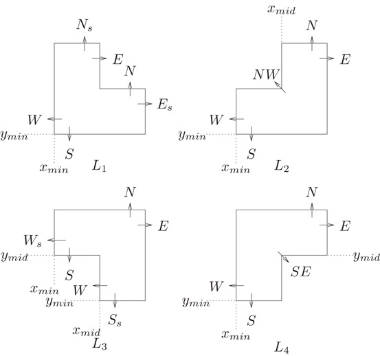
Figure 53.9L-shapes and their pointers.
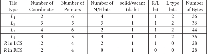
Figure 53.10Space requirements of tiles in LCS and RCS.
53.5.4.1Rectilinear Polygons
Since, in practice, circuit components can be arbitrary rectilinear polygons, it is necessary to partition them into rectangles to enable them to be stored in the corner stitching format. MAGIC handles this by using horizontal lines to partition the polygons. This is not necessary from a theoretical standpoint, but it simplifies the implementation of the various corner stitching operations. Nahar and Sahni [15] studied this problem and presented an O(n + kv log kv) algorithm to decompose a polygon with n vertices and kv vertical inversions into rectangles using horizontal cuts only. (The number of vertical inversions of a polygon is defined as the minimum number of changes in vertical direction during a walk around the polygon divided by 2.) The quantity kv was observed to be small for polygons encountered in VLSI mask data. Consequently, the Nahar-Sahni algorithm outperforms an O(n log n) planesweep algorithm on VLSI mask data. We note that this problem is different from the problem of decomposing a rectilinear polygon into a minimum number of rectangles using both horizontal and vertical cuts, which has been studied extensively in the literature [16–19].
However, the extension is slower than the original corner stitching, and also harder to implement. Lopez and Mehta [20] presented algorithms for the problem of optimally breaking an arbitrary rectilinear polygon into L-shapes using horizontal cuts.
53.5.4.2Parallel Corner Stitching
Mehta and Wilson [21] have studied a parallel implementation of corner stitching. Their work focuses on two batched operations (batched insert and delete). Their approach results in a significant speed-up in run times for these operations.
53.5.4.3Comments about Corner Stitching
1.Corner stitching requires rectangles to be non-overlapping. A single layer of the chip consists of non-overlapping rectangles, but all the layers taken together will consist of overlapping rectangles. So, an instance of the corner stitching data structure can only be used for a single layer. However, corner stitching can be used to store multiple layers in the following way: consider two layers A and B. Superimpose the two layers. This can be thought of as a single layer with four types of rectangles: vacant rectangles, type A rectangles, type B rectangles, and type AB rectangles. Unfortunately, this could greatly increase the number of rectangles to be stored. It also makes it harder to perform insertion and deletion operations. Thus, in MAGIC, the layout is represented by a number of single-layer corner stitching instances and a few multiple-layer instances when the intersection between rectangles in different layers is meaningful; for example, transistors are formed by the intersection of poly and diffusion rectangles.
2.Corner stitching is difficult to implement. While the data structure itself is quite elegant, the author’s experience is that its implementation requires one to consider a lot of details that are not considered in a high-level description. This is supported by the following remark attributed to John Ousterhout [13]:
Corner-stitching is pretty straightforward at a high level, but it can become much more complicated when you actually sit down to implement things, particularly if you want the implementation to run fast
3.The Point Find operation can be slow. For example, Point Find could visit all the tiles in the data structure resulting in an O(n) time complexity. On the average, it requires time. This is expensive when compared with the O(log n) complexity that may be possible by using a tree type data structure. From a practical standpoint, the slow speed may be tolerable in an interactive environment in which a user performs one operation at a time (e.g., a Point Find could be performed by a mouse button click). Here, a slight difference in response time might not be noticeable by the user. Furthermore, in an interactive environment, these operations might actually be fast because they take advantage of locality of reference (i.e., the high likelihood that two successive points being searched by a user are near each other in the layout). However, in batch mode, where a number of operations are performed without user involvement, one is more likely to experience the average case complexity (unless the order of operations is chosen carefully so as to take advantage of locality of reference). The difference in time between corner stitching and a faster logarithmic technique will be significant.
4.Corner stitching requires more memory to store vacant tiles.
Quad trees have been considered in Chapters 17 and 20. These chapters demonstrate that there are different flavors of quad-trees depending on the type of the data that are to be represented. For example, there are quad trees for regions, points, rectangles, and boundaries. In this chapter, we will be concerned with quad-trees for rectangles. We also note that Chapter 19 describes several data structures that can be used to store rectangles. To the best of my knowledge, the use of these structures has not been reported in the VLSI design automation literature.
The underlying principle of the quad tree is to recursively subdivide the two-dimensional layout area into four “quads” until a stopping criterion is satisfied. The resulting structure is represented by a tree with a node corresponding to each quad, with the entire layout area represented by the root. A node contains children pointers to the four nodes corresponding the quads formed by the subdivision of the node’s quad. Quads that are not further subdivided are represented by leaves in the quad tree.
Ideally, each rectangle is the sole occupant of a leaf node. In general, of course, a rectangle does not fit inside any leaf quad, but rather intersects two or more leaf quads. To state this differently, it may intersect one or more of the horizontal and vertical lines (called bisectors) used to subdivide the layout region into quads. Three strategies have been considered in the literature as to where in the quad tree these rectangles should be stored. These strategies, which have given rise to a number of quad tree variants, are listed below and are illustrated in Figure 53.11.
1.SMALLEST: Store a rectangle in the smallest quad (not necessarily a leaf quad) that contains it. Such a quad is guaranteed to exist since each rectangle must be contained in the root quad.
2.SINGLE: Store a rectangle in precisely one of the leaf quads that it intersects.
3.MULTIPLE: Store a rectangle in all of the leaf quads that it intersects.
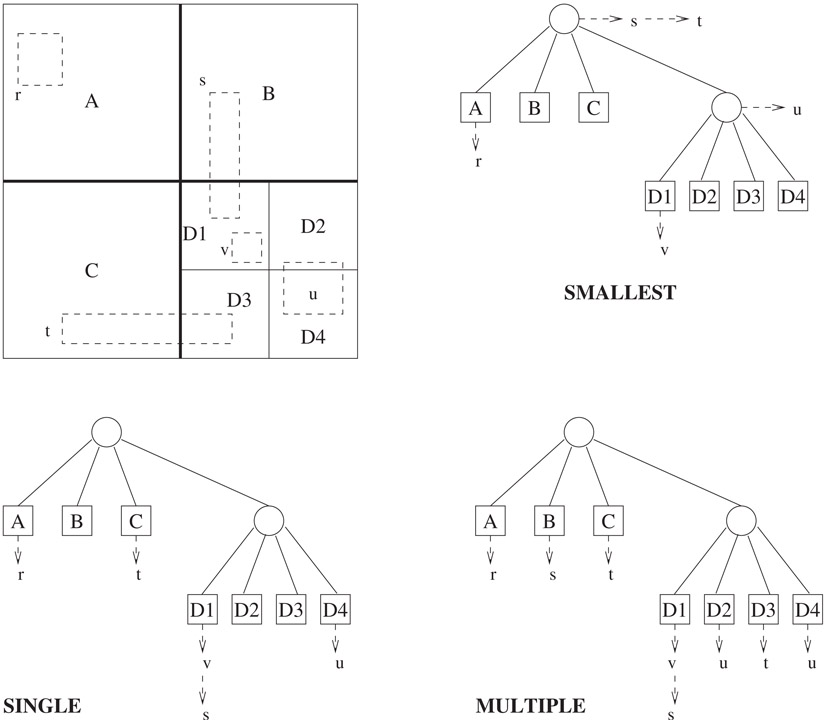
Figure 53.11Quadtree variations.
Obviously, if there is only one rectangle in a quad, there is no need to further subdivide the quad. However, this is an impractical (and sometimes impossible) stopping criterion. Most of the quad tree variants discussed below have auxiliary stopping criteria. Some subdivide a quad until it reaches a specified size related to the typical size of a small rectangle. Others stop if the number of rectangles in a quad is less than some threshold value. Figure 53.12 lists and classifies the quad tree variants.
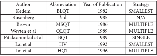
Figure 53.12Summary of Quad-tree variants.
53.6.1Bisector List Quad Trees
Bisector List Quad Trees (BLQT) [22], which was the first quad-tree structure proposed for VLSI layouts, used the SMALLEST strategy. Here, a rectangle is associated with the smallest quad (leaf or non-leaf) that contains it. Any non-leaf quad Q is subdivided into four quads by a vertical bisector and a horizontal bisector. Any rectangle associated with this quad must intersect one or both of the bisectors (otherwise, it is contained in one of Q’s children, and should not be associated with Q). The set of rectangles are partitioned into two sets: V, which consists of rectangles that intersect the vertical bisector and H, which consists of rectangles that intersect the horizontal bisector. Rectangles that intersect both bisectors are arbitrarily assigned to one of V and H. These “lists” were actually implemented using binary trees. The rationale was that since most rectangles in IC layouts were small and uniformly distributed, most rectangles will be at leaf quads. A region search operation identifies all the quads that intersect a query window and checks all the rectangles in each of these quads for intersection with the query window. The BLQT (which is also called the MX-CIF quadtree) is also described in Chapter 17.
Rosenberg [23] compared BLQT with k-d trees and showed experimentally that k-d trees outperformed an implementation of BLQT. Rosenberg’s implementation of the BLQT differs from the original in that linked lists rather than binary trees were used to represent bisector lists. It is hard to evaluate the impact of this on the experimental results, which showed that point-find and region-search queries visit fewer nodes when the k-d tree is used instead of BLQT. The experiments also show that k-d trees consume about 60%–80% more space than BLQTs.
53.6.3Multiple Storage Quad Trees
In 1986, Brown proposed a variation [24] called Multiple Storage Quad Trees (MSQT). Each rectangle is stored in every leaf quad it intersects. (See the quad tree labeled “MULTIPLE” in Figure 53.11.) An obvious disadvantage of this approach is that it results in wasted space. This is partly remedied by only storing a rectangle once and having all of the leaf quads that it intersects contain a pointer to the rectangle. Another problem with this approach is that queries such as Region Search may report the same rectangle more than once. This is addressed by marking a rectangle when it is reported for the first time and by not reporting rectangles that have been previously marked. At the end of the Region Search operation, all marked rectangles need to be unmarked in preparation for the next query. Experiments on VLSI mask data were used to evaluate MSQT for different threshold values and for different Region Search queries. A large threshold value results in longer lists of pointers in the leaf quads that have to be searched. On the other hand, a small threshold value results in a quad-tree with greater height and more leaf nodes as quads have to be subdivided more before they meet the stopping criterion. Consequently, a rectangle now intersects and must be pointed at by more leaf nodes. A Region Search query with a small query rectangle (window) benefits from a smaller threshold because it has to search smaller lists in a handful of leaf quads. A large window benefits from a higher threshold value because it has to search fewer quads and encounters fewer duplicates.
In 1989, Weyten and De Pauw [25] proposed a more efficient implementation of MSQT called Quad List Quad Trees (QLQT). For Region Searches, experiments on VLSI data showed speedups ranging from 1.85 to 4.92 over MSQT, depending on the size of the window. In QLQT, four different lists (numbered 0–3) are associated with each leaf node. If a rectangle intersects the leaf quad, a pointer to it is stored in one of the four lists. The choice of the list is determined by the relative position of this rectangle with respect to the quad. The relative position is encoded by a pair of bits xy. x is 0 if the rectangle does not cross the lower boundary of the leaf quad and is 1, otherwise. Similarly, y is 0 if the rectangle does not cross the left boundary of the leaf quad and is 1, otherwise. The rectangle is stored in the list corresponding to the integer represented by this two bit string. Figure 53.13 illustrates the concept. Notice that each rectangle belongs to exactly one list 0. This corresponds to the quad that contains the bottom left corner of the rectangle. Observe, also, that the combination of the four lists in a leaf quad gives the same pointers as the single list in the same leaf in MSQT. The Region Search of MSQT can now be improved for QLQT by using the following procedure for each quad that intersects the query window: if the query window’s left edge crosses the quad, only the quad’s lists 0 and 1 need to be searched. If the window’s bottom edge crosses the quad, the quad’s lists 0 and 2 need to be searched. If the windows bottom left corner belongs to the quad, all four lists must be searched. For all other quads, only list 0 must be searched. Thus the advantages of the QLQT over MSQT are:
1.QLQT has to examine fewer list nodes than MSQT for a Region Search query.
2.Unlike MSQT, QLQT does not require marking and unmarking procedures to identify duplicates.
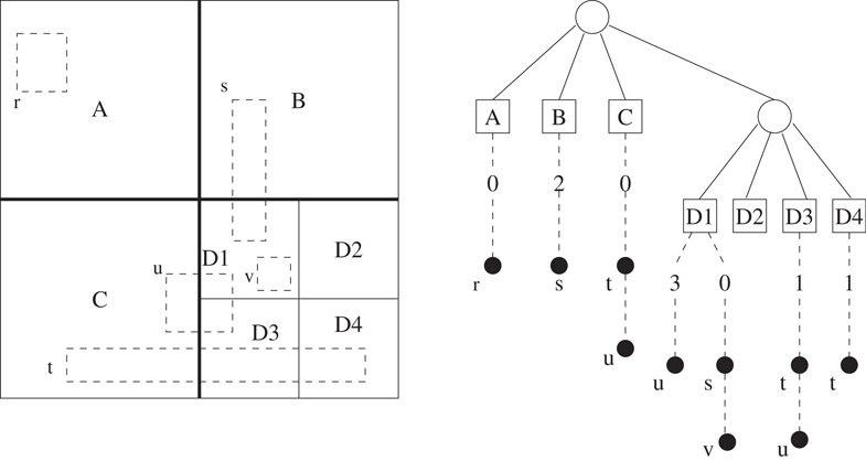
Figure 53.13The leaf quads are A, B, C, D1, D2, D3, and D4. The rectangles are r − v. Rectangle t intersects quads C, D3, and D4 and must appear in the lists of each of the leaf nodes in the quad tree. Observe that t does not cross the lower boundaries of any of the three quads and x = 0 in each case. However, t does cross the left boundaries of D3 and D4 and y = 1 in these cases. Thus t goes into list 1 in D3 and D4. Since t does not cross the left boundary of C, it goes into list 0 in C. Note that the filled circles represent pointers to the rectangles rather than the rectangles themselves.
Later, in 1989, Pitaksanonkul et al. proposed a variation of quad trees [26] that we refer to as Bounded Quad Trees (BQT). Here, a rectangle is only stored in the quad that contains its bottom left corner. (See the quad tree labeled “SINGLE” in Figure 53.11.) This may be viewed as a version of QLQT that only uses list 0. Experimental comparisons with k-d trees show that for small threshold values, quad trees search fewer nodes than k-d trees.
Next, in 1993, Lai et al. [27] presented a variation that once again uses bisector lists. It overcomes some of the inefficiencies of the original BLQT by a tighter implementation: An HV Tree consists of alternate levels of H-nodes and V-nodes. An H node splits the space assigned to it into two halves with a horizontal bisector while a V-node does the same by using a vertical bisector. A node is not split if the number of rectangles assigned to it is less than some fixed threshold.
Rectangles intersecting an H node’s horizontal bisector are stored in the node’s bisector list. Bisector lists are implemented using cut trees. A vertical cutline divides the horizontal bisector into two halves. All rectangles that intersect this vertical cutline are stored in the root of the cut tree. All rectangles to the left of the cutline are recursively stored in the left subtree and all rectangles to the right are recursively stored in the right subtree. So far, the data structure is identical to Kedem’s binary tree implementation of the bisector list. In addition to maintaining a list of rectangles intersecting a vertical cutline at the corresponding node n, the HV tree also maintains four additional bounds which significantly improve performance of the Region Search operation. The bounds y_upper_bound and y_lower_bound are the maximum and minimum y coordinates of any of the rectangles stored in n or in any of n’s descendants. The bounds x_lower_bound and x_upper_bound are the minimum and maximum x coordinates of the rectangles stored in node n. Figure 53.14 illustrates these concepts. Comprehensive experimental results comparing HVT with BQT, kD, and QLQT showed that the data structures ordered from best to worst in terms of space requirements were HVT, BQT, kD, and QLQT. In terms of speed, the best data structures were HVT and QLQT followed by BQT and finally kD.
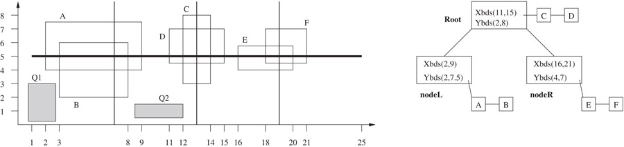
Figure 53.14Bisector list implementation in HVT. All rectangles intersect the thick horizontal bisector line (y = 5). The first vertical cutline at x = 13 corresponding to the root of the tree intersects rectangles C and D. These rectangles are stored in a linked list at the root. Rectangles A and B are to the left of the vertical cutline and are stored in the left subtree. Similarly, rectangles C and D are stored in the right subtree. The X bounds associated with the root node are obtained by examining the x coordinates of rectangles C and D, while its Y bounds are obtained by examining the y coordinates of all six rectangles stored in the tree. The two shaded rectangles are query rectangles. For Q1, the search will start at Root, but will not search the linked list with C and D because Q1’s right side is to the left of Root’s lower x bound. The search will then examine nodeL, but not nodeR. For Q2, the search will avoid searching the bisector list entirely because its upper side is below Root’s lower y bound.
In 1997, Lai et al. [28] described a variation of the QLQT that was specifically designed for design rule checking. Design-rule checking requires one to check rectangles in the vicinity of the query rectangle for possible violations. Previously, this was achieved by employing a traditional region query whose rectangle was the original query rectangle extended in all directions by a specified amount. Region searches start at the root of the tree and proceed down the tree as discussed previously. The hinted quadtree is based on the philosophy that it is wasteful to begin searching at the root, when, with an appropriate hint, the algorithm can start the search lower down in the tree. Two questions arise here: at which node should the search begin and how does the algorithm get to that node? The node at which the design rule check for rectangle r begins is called the owner of r. This is defined as the lowest node in the quad-tree that completely contains r expanded in all four directions. Since the type of r is known (e.g., whether it is n-type diffusion or metal), the amount by which r has to be expanded is also known in advance. Clearly, any rectangle that intersects the expanded r must be referenced by at least one leaf in the owner node’s subtree. The owner node may be reached by following parent pointers from the rectangle. However, this could be expensive. Consequently, in HQT, each rectangle maintains a pointer to the owner virtually eliminating the cost of getting to that node. Although this is the main contribution of the HQT, there are additional implementation improvements over the underlying QLQT that are used to speed up the data structure. First, the HQT resolves the situation where the boundary of a rectangle stored in the data structure or a query rectangle coincides with that of a quad. Second, HQT sorts the four lists of rectangles stored in each leaf node with one of their x or y coordinates as keys. This reduces the search time at the leaves and consequently makes it possible to use a higher threshold than that used in QLQT. Experimental results showed that HQT out-performs QLQT, BQT, HVT, and k-d on neighbor-search queries by at least 20%. However, its build-time and space requirements were not as good as some of the other data structures.
Most of the research in VLSI layout data structures was carried out in the early 80s through the mid-90s. This area has not been very active since then. One reason is that there continue to be several important challenges in VLSI physical design automation that must be addressed quickly so that physical design does not become a bottleneck to the continuing advances in semiconductors predicted by Moore’s Law. These challenges require physical design tools to consider “deep sub-micron effects” into account and take priority over data structure improvements. The implication of these effects is that problems in VLSI physical design are no longer purely geometric, but rather need to merge geometry with electronics. For example, in the early 1980s, one could safely use the length of a wire to estimate the delay of a signal traveling along it. This is no longer true for the majority of designs. Thus, the delay of a signal along the wire must now be estimated by factoring in its resistance and capacitance, in addition to its geometry. On the other hand, the more detailed computations of electronic quantities like capacitance, resistance, and inductance require the underlying data structures to support more complex operations. Thus, the author believes that there remain opportunities for developing better layout data structures. Another area that, to the best of our knowledge, has been neglected in the academic literature is that VLSI layout data needs to be efficiently stored in secondary storage because of its sheer size. Thus, although there is potential for academic research in this area, we believe that the design automation industry may well have addressed these issues in their proprietary software.
Unlike corner stitching, quad-trees permit rectangles to overlap. This addresses the problem that corner stitching has with handling multiple layers. On the other hand, corner stitching was designed for use in the context of an interactive layout editor, whereas quad trees are designed in the context of batched operations. We note that, to our knowledge, relatively recent data structures such as R trees have not been used for VLSI layout. It is unclear what the outcome of this comparison will be. On one hand, R-trees are considered to be faster than quad trees. On the other, the quad-trees developed in VLSI have been improved and optimized significantly as we have seen in this chapter. Also, VLSI data has generally been considered to consist of uniformly small rectangles, which may make it particularly suitable for quad trees, although this property may not be true when wires are considered.
This work was supported, in part, by the National Science Foundation under grant CCR-9988338.
1.N. Sherwani, Algorithms for VLSI Physical Design Automation. Boston: Kluwer Academic Publishers, 1992.
2.M. Sarrafzadeh and C. K. Wong, An Introduction to VLSI Physical Design. New York: McGraw Hill, 1996.
3.S. Sait and H. Youssef, VLSI Physical Design Automation: Theory and Practice. Piscataway, NJ: IEEE Press, 1995.
4.N. H. E. Weste and K. Eshraghian, Principles of CMOS VLSI Design: A Systems Perspective, Second Edition. New York: Addison Wesley, 1993.
5.J. L. Hennessy and D. A. Patterson, Computer Architecture: A Quantitative Approach, Third Edition. New York: Morgan Kaufmann, 2003.
6.D. G. Boyer, “Symbolic Layout Compaction Review,” in Proceedings of 25th Design Automation Conference, Anaheim, CA, pp. 383–389, 1988.
7.J. Ousterhout, G. Hamachi, R. Mayo, W. Scott, and G. Taylor, “Magic: A VLSI Layout System,” in Proc. of 21st Design Automation Conf., Albuquerque, New Mexico, pp. 152–159, 1984.
8.J. K. Ousterhout, “Corner Stitching: A Data Structuring Technique for VLSI Layout Tools,” IEEE Transactions on Computer-Aided Design, vol. 3, no. 1, pp. 87–100, 1984.
9.D. P. Mehta, “Estimating the Memory Requirements of the Rectangular and L-Shaped Corner Stitching Data Structures,” ACM Transactions on the Design Automation of Electronic Systems, vol. 3, no. 2, pp. 272–284, 1998.
10.D. P. Mehta, “CLOTH_MEASURE: A Software Tool for Estimating the Memory Requirements of Corner Stitching Data Structures,” VLSI Design, vol. 7, no. 4, pp. 425–436, 1998.
11.M. Quayle and J. Solworth, “Expanded Rectangles: A New VLSI Data Structure,” in ICCAD, Santa Clara, California, pp. 538–541, 1988.
12.D. Marple, M. Smulders, and H. Hegen, “Tailor: A Layout System Based on Trapezoidal Corner Stitching,” IEEE Transactions on Computer-Aided Design, vol. 9, no. 1, pp. 66–90, 1990.
13.C. H. Séquin and H. da Silva Façanha, “Corner Stitched Tiles with Curved Boundaries,” IEEE Transactions on Computer-Aided Design, vol. 12, no. 1, pp. 47–58, 1993.
14.D. P. Mehta and G. Blust, “Corner Stitching for Simple Rectilinear Shapes,” IEEE Transactions on Computer-Aided Design of Integrated Circuits and Systems, vol. 16, 186–198, Feb. 1997.
15.S. Nahar and S. Sahni, “A Fast Algorithm for Polygon Decomposition,” IEEE Transactions on Computer-Aided Design, vol. 7, 478–483, Apr. 1988.
16.T. Ohtsuki, “Minimum Dissection of Rectilinear Regions,” in Proceedings 1982 International Symposium on Circuits and Systems (ISCAS), Rome, Italy, pp. 1210–1213, 1982.
17.H. Imai and T. Asano, “Efficient Algorithms for Geometric Graph Search Algorithms,” SIAM Journal on Computing, vol. 15, 478–494, May 1986.
18.W. T. Liou, J. J. M. Tan, and R. C. T. Lee, “Minimum Partitioning of Simple Rectilinear Polygons in O(n loglog n) Time,” in Proceedings of the Fifth Annual Symposium on Computational Geometry, Saarbruchen, Germany, pp. 344–353, 1989.
19.S. Wu and S. Sahni, “Fast Algorithms to Partition Simple Rectilinear Polygons,” International Journal on Computer Aided VLSI Design, vol. 3, 241–270, 1991.
20.M. Lopez and D. Mehta, “Efficient Decomposition of Polygons into L-Shapes with Applications to VLSI Layouts,” ACM Transactions on Design Automation of Electronic Systems, vol. 1, 371–395, 1996.
21.D. Mehta and E. Wilson, “Parallel Algorithms for Corner Stitching,” Concurrency: Practice and Experience, vol. 10, 1317–1341, 1998.
22.G. Kedem, “The Quad-CIF Tree: A Data Structure for Hierarchical On-Line Algorithms,” in Proceedings of the 19th Design Automation Conference, Piscataway, NJ, pp. 352–357, 1982.
23.J. B. Rosenberg, “Geographical Data Structures Compared: A Study of Data Structures Supporting Region Queries,” IEEE Transactions on Computer-Aided Design, vol. 4, no. 1, pp. 53–67, 1985.
24.R. L. Brown, “Multiple Storage Quad Trees: A Simpler Faster Alternative to Bisector List Quad Trees,” IEEE Transactions on Computer-Aided Design, vol. 5, no. 3, pp. 413–419, 1986.
25.L. Weyten and W. de Pauw, “Quad List Quad Trees: A Geometric Data Structure with Improved Performance for Large Region Queries,” IEEE Transactions on Computer-Aided Design, vol. 8, no. 3, pp. 229–233, 1989.
26.A. Pitaksanonkul, S. Thanawastien, and C. Lursinsap, “Comparison of Quad Trees and 4-D Trees: New Results,” IEEE Transactions on Computer-Aided Design, vol. 8, no. 11, pp. 1157–1164, 1989.
27.G. Lai, D. S. Fussell, and D. F. Wong, “HV/VH Trees: A New Spatial Data Structure for Fast Region Queries,” in Proceedings of the 30th Design Automation Conference, Dallas, TX, pp. 43–47, 1993.
28.G. Lai, D. S. Fussell, and D. F. Wong, “Hinted Quad Trees for VLSI Geometry DRC Based on Efficient Searching for Neighbors,” IEEE Transactions on Computer-Aided Design, vol. 15, no. 3, pp. 317–324, 1996.
*This chapter has been reprinted from first edition of this Handbook, without any content updates.