
Floorplan Representation in VLSI*
Zhou Feng
Fudan University
Bo Yao
University of California, San Diego
Chung-Kuan Cheng
University of California, San Diego
Statement of Floorplanning Problem•Motivation of the Representation•Combinations and Complexities of the Various Representations•Slicing, Mosaic, LB Compact, and General Floorplans
54.2Graph Based Representations
Constraint Graphs•Corner Stitching•Twin Binary Tree•Single Tree Representations
54.3Placement Based Representations
Sequence-Pair•Bounded-Sliceline Grid•Corner Block List•Slicing Tree
54.4Relationships of the Representations
Summary of the Relationships•A Mosaic Floorplan Example•A General Floorplan Example
54.5Rectilinear Shape Handling
There are two main data models that can be used for representing floorplans: graph-based and placement based [23–29].
The graph-based approach includes constraint graphs, corner stitching, twin binary tree, and O-tree. They utilize constraint graphs or their simplified versions directly for the encoding. Constraint graphs are basic representations. The corner stitching simplifies the constraint graph by recording only the four neighboring blocks to each block. The twin binary tree then reduces the recorded information to only two neighbors of each block, and organizes the neighborhood relations in a pair of binary trees. The O-tree is a further simplification to the twin binary tree. It keeps only one tree for encoding.
The placement-based representations use the relative positions between blocks in a placement for encoding. This category includes sequence pair, bounded-sliceline grid, corner block list and slicing trees. The sequence pair and bounded-sliceline grid can be applied to general floorplan. The corner block list records only the relative position of adjacent blocks, and is available to mosaic floorplan only. The slicing trees are for slicing floorplan, which is a type of mosaic floorplan. The slicing floorplan can be constructed by hierarchical horizontal or vertical merges and thus can be captured by a binary tree structure known as the slicing tree.
The rest of this chapter is organized as follows. In Section 54.1, we give the introduction and the problem statement of floorplanning. In Section 54.2, we discuss the graph-based representations. In Section 54.3, we introduce the placement-based representations. We describe the relationship between different representations in Section 54.4. We illustrate the shape handling of rectilinear blocks in Section 54.5 and summarize the chapter in Section 54.6.
54.1.1Statement of Floorplanning Problem
Today’s complexity in circuitry design wants a hierarchical approach [1]. The entire circuit is partitioned into several sub-circuits, and the sub-circuits are further partitioned into smaller sub-circuits, until they are small enough to be handled. The relationship between the sub-circuits can be represented with a tree as shown in Figure 54.1. Here every sub-circuit is called a block, and hence the entire circuit is called the top block. From the layout point of view, every block corresponds to a rectangle, which contains sub-blocks or directly standard cells. Among the decisions to be made is the determination of shape (aspect ratio) and the pin positions on the blocks. In the top-down hierarchical methodology, blocks are designed from the top block (the entire circuit) to the leaf blocks (small modules). The minimizations of chip area and wire length are the basic targets for any layout algorithm. In addition, there are case-dependent constraints that will influence the layouts, such as the performance, the upper or/and lower boundaries of aspect ratio, the directions of pins, etc.
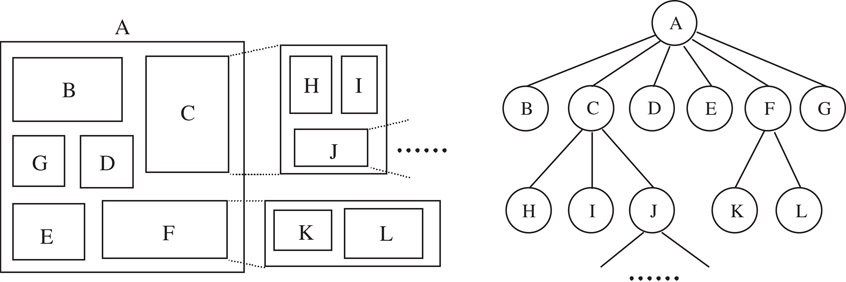
Figure 54.1Hierarchical structure of blocks.
Now we give the definition of floorplanning problem:
Inputs:
1.The net-lists of the sub-circuits;
2.The area estimation of blocks and, if any, the aspect ratio constraints on the blocks;
3.The target area and shape of the entire chip.
Outputs:
1.The shapes and positions of blocks;
2.The pin positions on the blocks.
The objective functions involve: the chip area, the total wire length and, if any, the performances.
54.1.2Motivation of the Representation
Floorplan representation becomes an important issue in floorplanning for the following reasons.
1.The blocks may have arbitrary shapes and locations, while the size of memory used to represent a two-dimensional floorplan should be O(n).
2.For the general floorplanning problem, iterative improvement is the commonly used approach. The search for the best solution has proven to be NP-complete, so many heuristic optimizing algorithms, such as dynamic programming, simulated annealing, zone refinement, cluster refinement, have been adopted. The representation should also facilitate the operations called by those optimizing algorithms.
3.The storage resources requirement, the redundancy of the representation and the complexity of translating the representation into floorplan are always the concerns in floorplanning. Here redundancy refers to the situation that several different expressions actually correspond to the same physical layout. Essentially, a heuristic algorithm searches part of the solution space to find the local optimal solution, which is hopefully very close to the global optimal solution. Redundancy causes the optimizing algorithm evaluate the same floorplan repeatedly.
54.1.3Combinations and Complexities of the Various Representations
The number of possible floorplan representations describes how large the searching space is. It also discloses the redundancy of the representation. For general floorplans with n blocks, the combinations of the various representations are listed in Table 54.1. Note that the twin binary tree representation has a one to one relation with the mosaic floorplan, and the slicing tree has a one to one relation with the slicing floorplan [2]. In other words, for these two representations, the number of combinations is equal to the number of possible floorplan configurations and there is no redundancy.
Table 54.1Combinations of the Representations
|
Representation |
Combinations |
|
Twin binary tree |
n!*B(n), where |
|
O-Tree |
O() |
|
Sequence pair |
(n!)2 |
|
Bounded-sliceline grid |
|
|
Corner block list |
O() |
|
Slicing tree |
n!*A(n − 1), where A(n) is the super-Catalan number with the following definition: |
|
A(0) = A(1) = 1 and A(n) = (3(2n − 3)A(n − 1) − (n − 3)A(n − 2))/n |
The combination numbers of sequence pairs, mosaic floorplans, slicing floorplans, and O-trees are illustrated on a log scale in Figure 54.2. The combination numbers are normalized by n!, which is the number of permutations of n blocks. The slopes of the lines for mosaic floorplans, slicing floorplans, and O-tree structures are the constants 0.89, 0.76, and 0.59, respectively. On the other hand, the slope of the line for sequence pair increases with a rate of log n. Table 54.2 provides the exact numbers of the combinations for the floorplans or representations with the block number ranging from 1 to 17.
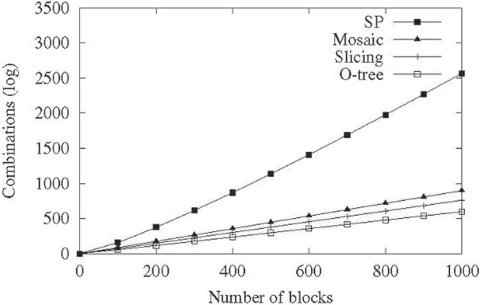
Figure 54.2Combination of floorplans and representations.
Table 54.2Exact Number of Combinations of Different Floorplan Configurations and Representations
|
Number of Blocks |
Combinations of O-Tree |
Combinations of Slicing Floorplan |
Combinations of Mosaic Floorplan |
Combinations of Sequence Pairs |
|
1 |
1 |
1 |
1 |
1 |
|
2 |
2 |
2 |
2 |
2 |
|
3 |
5 |
6 |
6 |
6 |
|
4 |
14 |
22 |
22 |
24 |
|
5 |
42 |
90 |
92 |
120 |
|
6 |
132 |
394 |
422 |
720 |
|
7 |
429 |
1806 |
2074 |
5040 |
|
8 |
1430 |
8558 |
10,754 |
40,320 |
|
9 |
4862 |
41,586 |
58,202 |
362,880 |
|
10 |
16,796 |
206,098 |
326,240 |
3,628,800 |
|
11 |
58,786 |
1,037,718 |
1,882,690 |
39,916,800 |
|
12 |
208,012 |
5,293,446 |
11,140,560 |
479,001,600 |
|
13 |
742,900 |
27,297,738 |
67,329,992 |
6,227,020,800 |
|
14 |
2,674,440 |
142,078,746 |
414,499,438 |
87,178,291,200 |
|
15 |
9,694,845 |
745,387,038 |
2,593,341,586 |
1,307,674,368,000 |
|
16 |
35,357,670 |
3,937,603,038 |
16,458,756,586 |
20,922,789,888,000 |
|
17 |
129,644,790 |
20,927,156,706 |
105,791,986,682 |
355,687,428,096,000 |
The time complexities of the operations transforming a representation to a floorplan are very important, because they determine the efficiency of the floorplan optimizations. The complexities of the representations covered in this chapter are compared in Table 54.3, where n is the number of blocks in a floorplan.
Table 54.3Time Complexity Comparison of the Representations
|
Representation |
From a Representation to a Floorplan |
|
Constraint graph |
O(n) |
|
Corner stitching |
O(n) |
|
Twin binary tree |
O(n) |
|
O-Tree |
O(n) |
|
Sequence pair |
O(nloglogn) |
|
Bounded-sliceline grid |
O(n2) |
|
Corner block list |
O(n) |
|
Slicing tree |
O(n) |
For sequence-pair, the time complexity to derive a floorplan is O(nloglogn) due to a fast algorithm proposed in Reference 3. We will discuss more on this in Section 54.3.1 For bounded slicing grid, there is a trade off between the solution space and the time complexity of deriving a floorplan. To ensure that the solution space covers all the optimal solutions, we need the grid size to be at lease n by n. This results in an O(n2) time complexity in deriving a floorplan [4]. For the rest of the representations, there are algorithms with O(n) time complexity to convert them into constraint graphs. The time complexity to derive a floorplan is thus O(n).
54.1.4Slicing, Mosaic, LB Compact, and General Floorplans
A layout can be classified as a slicing floorplan if we can partition the chip with recursive horizontal or vertical cut lines (Figure 54.3a). In a mosaic floorplan, the chip is partitioned by horizontal and vertical segments into rectangular regions and each region corresponds to exactly one block (Figure 54.3b). For a general floorplan, we may find empty space outside rectangular block regions (Figure 54.3c). An LB-compact floorplan is a restricted general floorplan in that all blocks are shifted to their left and bottom limits. In summary, the set of general floorplans covers the set of LB-compact floorplans, which covers the set of mosaic floorplans, and which covers the set of slicing floorplans (Figure 54.4).
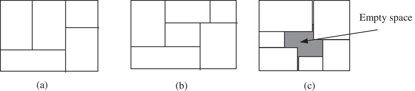
Figure 54.3(a) Slicing floorplan; (b) Mosaic floorplan; (c) General floorplan.
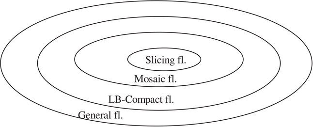
Figure 54.4Set coverage of slicing floorplan, mosaic floorplans, LB-compact floorplans and general floorplans.
For slicing and mosaic floorplans, the vertical segments define the left-right relation among the separated regions, and the horizontal segments define the above-below relation. Suppose that we shift the segments to change the sizes of the regions, we view the new floorplan to be equivalent to the original floorplan in terms of their topologies [5–7]. Therefore, we can devise representations to define the topologies of slicing and mosaic floorplans independent of the sizes of the blocks (Figure 54.3a and b). In contrast, for a general floorplan, it is rather difficult to draw a meaningful layout (Figure 54.3c) without the knowledge of the block dimensions. One approach is to extend the mosaic floorplans to general floorplans by adding empty blocks [8]. It is shown that to convert a mosaic floorplan with n blocks into a general floorplan, the upper bound on the number of empty blocks inserted is . [8]
In a mosaic floorplan, two adjacent blocks meet at a T-junction by sharing the non-crossing edge of the junction. There are four directions of T-junctions as is illustrated in Figure 54.5. In the case of Figure 54.5a and b, block B is termed the C-neighbor at the lower left corner of block A. In Figure 54.5c and d, block B is the C-neighbor at the upper right corner of block A. The C-neighbor is used to construct twin binary tree representation.
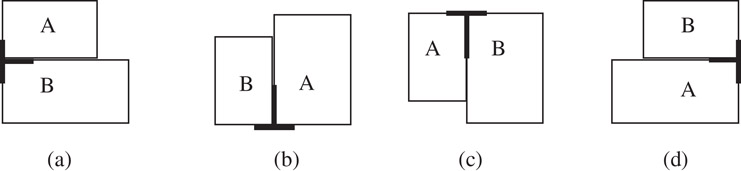
Figure 54.5Four directions of T-junctions.
The degeneration of a mosaic floorplan refers to the phenomenon that two T-junctions meet together to make up a cross-junction, as illustrated in Figure 54.6a. Some representations forbid the occurrence of degeneration. One scheme to solve the problem is to break one of the intersecting lines and assume a slight shift between the two segments, as shown in Figure 54.6b. Thus the degeneration disappears.
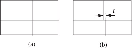
Figure 54.6Degeneration.
We generate an LB compact floorplan by compacting all blocks toward left and bottom. For a placement, suppose no block can be moved left, the placement is called L-compact. Similarly, if no block can be moved down, the placement is called B-compact. A floorplan is LB-compact if it is both L-compact and B-compact (Figure 54.7).
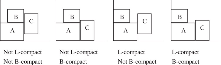
Figure 54.7Examples of L-compact and B-compact.
54.2Graph Based Representations
Graph based representations include constraint graphs, corner stitching, twin binary trees, and O-tree. They all utilize the constraint graphs or their simplified version for floorplan encoding.
Constraint graphs are directed acyclic graphs representing the adjacency relations between the blocks in a floorplan. In this subsection, we first define the constraint graphs for general floorplans. We then show that for mosaic floorplan, the constraint graphs have nice properties of triangulation and duality.
54.2.1.1The Generation of Constraint Graphs
Constraint graphs reflect the relative positions between blocks [9]. Constraint graphs can be applied to general floorplans, as is shown in Figure 54.8. A node in the constraint graph represents a block. A directed edge denotes the location relationship between two blocks. For example, A→B means block A is to the left of B in a horizontal constraint graph (Figure 54.8b). A→E means block A is on top of E in a vertical constraint graph (Figure 54.8c). Here we imply that if A→B and B→C, then A→C. Thus even though block A stands to the left of C, the edge between A and C is not necessarily shown. To mark the four sides of the chip, we add the nodes labeled with “left,” “right,” “top” and “down.” A pair of horizontal and vertical constraints graphs can represent a floorplan. Every constraint graph, whether it is a horizontal one or a vertical one, is planar and acyclic. Figure 54.9 shows an example of the constraint graphs to a mosaic floorplan. Figure 54.9a is the mosaic floorplan. Figure 54.9b and c are the corresponding horizontal and vertical constraint graphs, respectively.
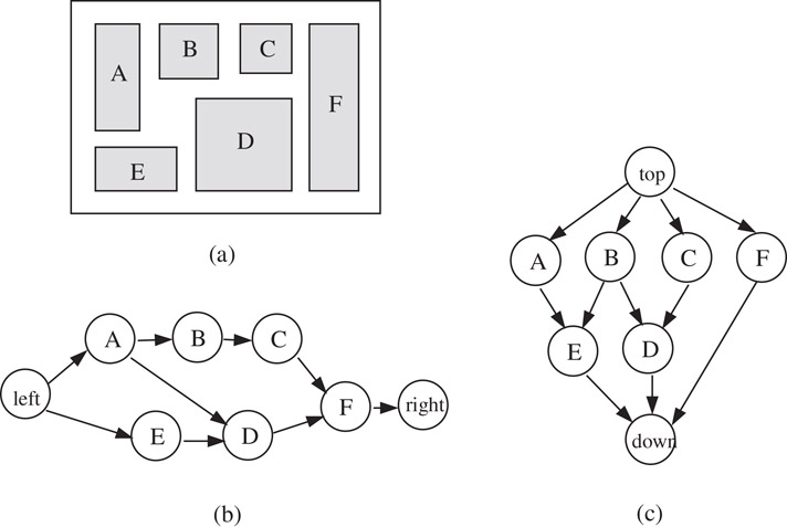
Figure 54.8Constraint graphs for a general floorplan.
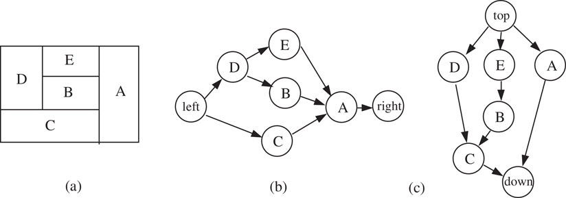
Figure 54.9Constraint graphs for a mosaic floorplan.
54.2.1.2Triangulation
For a mosaic floorplan without degeneration, if its horizontal and vertical constraint graphs are merged together, then we have the following conclusions [9]:
1.Every face is a triangle.
2.All internal nodes have a degree of at least 4.
3.All cycles, if not faces, have the length of at least 4.
Shown in Figure 54.10a is the result of merging the pair of constraint graphs in Figure 54.9. In fact, the merged constraint graph is a dual graph of its original floorplan (Figure 54.9b).
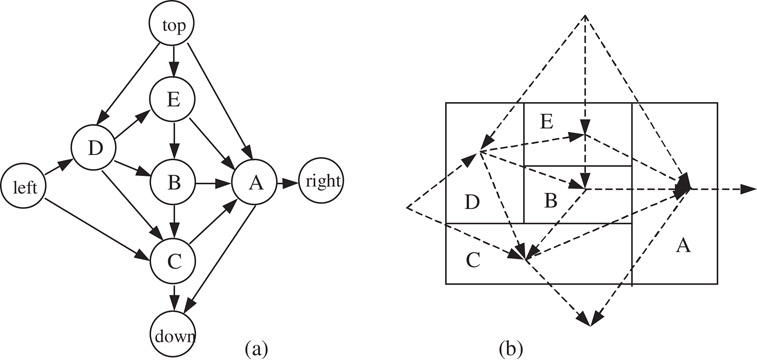
Figure 54.10Triangulation.
54.2.1.3Tutte’s Duality [10]
We can also build an edge-based constraint graph for a mosaic floorplan, where the nodes denote the lines separating the blocks while the edges denote the blocks. Labeling the lines with numbers (Figure 54.11a), we build a vertical constraint graph (Figure 54.11b) and a horizontal constraint graph (Figure 54.11c). Figure 54.11d demonstrates the result of merging the vertical and horizontal constraint graphs. Here, to make the merged graph clear, the edges representing horizontal constraints are drawn with dotted lines, and a letter at the intersection of a solid edge and a dotted edge denotes the two edges simultaneously. It is very interesting that, for mosaic floorplans, the vertical and horizontal constraint graphs are dual, as is called Tutte’s duality.

Figure 54.11Line-based constraint graphs.
Let’s see how Tutte’s duality is used to solve the sizing problem in floorplanning. We map the constraint graphs into circuit diagrams by replacing the edges in the vertical constraint graph with resistors, as illustrated in Figure 54.12.
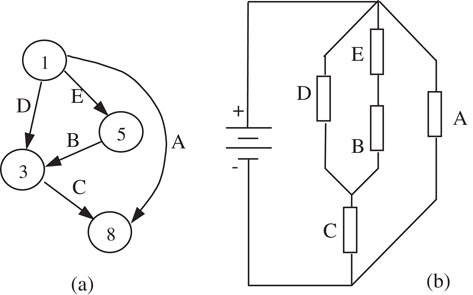
Figure 54.12Mapping a constraint graph to a circuit.
The circuit is subject to Kirchoff voltage law. As a result, taking Figure 54.12 as an example, we have:
Note that, if we denote the height and the width of block i to be Hi and Wi, we have (refer to Figure 54.12a):
By comparing the above two equation arrays, we can find that there is a perfect correspondence between the solutions of the circuit and the floorplan. Let us set the following assumptions: (only two of the three equations are independent)
Then we have:
Thus the theories dealing with large circuits can be borrowed to solve the sizing problem in floorplanning.
Constraint graphs have the advantages of being able to cope with any types of floorplans. However, it would be rather difficult to shift to a new floorplan with just a few simple operations on the graph. The efficiency is greatly discounted for the iteratively improving algorithms. Thus in Reference 11, a transitive closure graph (TCG) was proposed to simplify the rules of the operations. The relation of each pair of blocks is prescribed in either horizontal or vertical constraint graph via transitive closure, but not in both graphs.
Corner stitching is used to represent the topology of a mosaic floorplan. Simplified from constraint graphs, corner stitching [12] keeps only four pointers at the two opposite corners for every block. All the operations on a constraint graph can also be fulfilled on a corner stitching representation with acceptable increases in time complexity, while the storage for corner stitching becomes easier since the number of pointers attached to every block is fixed (equals to 4). Readers are referred to Chapter 53 for detailed descriptions and analyses of corner stitching.
Twin binary tree [2] representation applies to mosaic floorplans without degeneration. The twin binary tree is constructed as follows, every block takes its C-neighbor (Figure 54.5) as its parent. In the first tree, only the C-neighbors in lower left corners (Figure 54.5a and b) are taken into account. If the related T-junction is of type (a), then the block is a left child of its parent, and if the T-junction is of type (b), then the block is a right child. The most bottom-left block in the floorplan acts as the root of the tree. Similarly, in the second tree, the C-neighbors in upper right corners (Figure 54.12c and d) are used, and the most upper-right block becomes the tree’s root. Figure 54.13 gives an example of a twin binary tree.
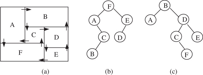
Figure 54.13Twin binary tree.
The pointers of twin binary trees are in fact a subset of those in corner stitching. Besides, It has been proved that twin binary tree is a non-redundant representation. In other words, every pair of trees corresponds to a unique mosaic floorplan.
The twin properties of binary trees can be illustrated with Figure 54.14. Consider the trees shown in Figure 54.13, we add a left child labeled “0” to every node without left child except the most left node, and a right child labeled “1” to every node without right child except the most right node. The resultant trees are the so-called extended trees (Figure 54.14). The sequences of the in-order traverse of the two extended trees shown in Figure 54.14 are “A0B1C1F0D1E” and “A1B0C0F1D0E” respectively. If we separate them into the label parts and the bit parts, we have π1 = ABCFDE, and α2 = 10010. It is interesting to find that and . So rather than store the two binary trees, we only keep the linear lists π and α in memory.
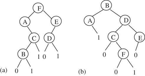
Figure 54.14Extended trees.
However, it is insufficient to recover the two binary trees just from π and α, so we need two more lists, β and β′. If the i-th element in π is the left child of its parent in the first tree or the root of the tree, we set the i-th element in β to be “0,” otherwise we set it “1.” In the similar way β′ is constructed according to the second tree. Thus we use a group of linear lists {π, α, β, β′}, called the twin binary sequence [8], to express the twin binary tree, and equivalently the floorplan.
Finally, we give the main properties of twin binary tree representation:
1.The memory required for storing the twin binary sequence is log2n + 3n − 1, because |π| = log2n, |α| = n − 1, and |β| = |β′| = n.
2.Twin binary tree is a non-redundancy floorplan representation.
3.The complexity of the translation between twin binary sequence and floorplan is O(n).
54.2.4Single Tree Representations
An ordered-tree (O-tree) [13,14], or equivalently the B* tree [15] representation uses a spanning tree of the constraint graph and the dimensions of the blocks. Because the widths and heights of the blocks are given, the representation can describe one kind of general floorplan termed LB-compact. With a proper encoding, a great enhancement on the storage efficiency and the perturbation easiness is obtained.
A horizontal O-tree is derived with the following rules:
1.If block A lies adjacent to the left side of block B, or, (here Xa is the coordinate of block A on the X-axis and Wa is the width of block A), then on the O-tree, B is A’s child. If there happens to exist more than one block adjacent to the left side of block B (satisfying the requirement ), one of them is assigned to be the parent of block B.
2.If block A lies on top of block B and the two blocks have the same parents on the O-tree, then B is A’s elder brother.
3.A virtual block is presumed to have the left most position, and therefore serves as the root of the O-tree.
Figure 54.15 shows an example of an O-tree representation for the same mosaic floorplan shown in Figure 54.13. If we show the pointer of every block pointing to its parent in the O-tree (Figure 54.15b), we can find that the pointers are in fact a subset of those in twin binary tree. Similarly a vertical O-tree can be built up. Without the loss of generality, hereafter we only discuss the horizontal O-tree.
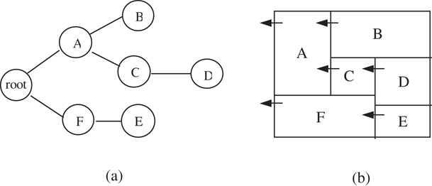
Figure 54.15Building an O-tree.
Next, let’s describe the O-tree with linear lists: a bit string (denoted with T) and a label string (denoted with π). The bit string records the structure of an O-tree. We make a depth-first traverse on the O-tree. A “0” is inserted into T for descending an edge while a “1” for ascending an edge. For example, the O-tree in Figure 54.16 corresponds to the bit string T = “001100011011.” Inversely, given the bit string, the structure of the O-tree is solely determined. To get the complete description of an O-tree, we need a second linear list, the label string, to record the labels of the tree’s nodes. Not only should the label string include all the labels of the tree’s nodes, but also reflect the labels’ positions on the tree. A depth-first traverse generates such a linear list. For the example in Figure 54.16, we have π = “FEACDB.”
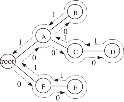
Figure 54.16Derivation of T, π.
Given a horizontal O-tree, or {T, π}, and the dimensions of blocks, the positions of blocks can be derived with the following rules:
1.Each block has to be placed to the left of its children.
2.If two blocks overlap along their x-coordinate projection, then the block having a higher index in π must be placed on top of the other one.
In fact the second rule applies to the situation in which none of the two blocks is a descendant of the other, like blocks “f” and “a,” or “b” and “d,” in Figure 54.16. The way we derive π indicates that the block with higher index always stands “higher.” To get to a placement, we need to locate all the blocks. The following operation is executed on blocks according to their orders in π. Here Bi refers to the i-th block, and refers to the coordinate of Bi’s left-bottom corner.
1.Find Bi’s parent, Bj, and then we have , here wj is the width of block Bj.
2.Let ψ be a set of blocks who have a lower index than Bi in π and have an projection overlap with Bi in the X-axis, find the maximum for Bk ∈ ψ, then we have .
Now we analyze the performance of O-tree:
1.The bit string has a length of 2n for an O-tree of n blocks, because each node except the root has an edge towards its parents and each edge is traversed twice during the construction of the bit string. The label string takes n log2n bits for we have to use log2n bits to distinguish the n blocks. So the total memory occupied by an O-tree is n(2 + log2n). By comparison, a sequence pair takes 2n log2n bits and a slicing structure takes n(6 + log2n) bits.
2.The time needed to transform {T, π} to a placement is linear to the number of blocks, or we can say the complexity of transforming {T, π} to a placement is O(n). For a sequence pair or a slicing structure, the complexity is or O(n) respectively. Upon this point, O-tree has the same performance as the slicing structure but is more powerful for representing a placement.
3.The number of combinations is , which is smaller than any other representation that has ever been discussed.
The floorplan of an arbitrarily given O-tree is not necessarily LB-compact. Yet in this case, we can compact the floorplan to reduce the chip area. Notice that an O-tree-to-placement transform tightens the blocks, with one direction having the priority. For example, in a placement transformed from a horizontal O-tree, the blocks are placed tighter along the X-axis than along the Y-axis. It would be undoubted that a placement transformed from a vertical O-tree will give Y-axis the priority. Thus, by iteratively making the transforms between horizontal O-trees and vertical O-trees via placements, we can finally reach an LB-compact floorplan (Figure 54.17).
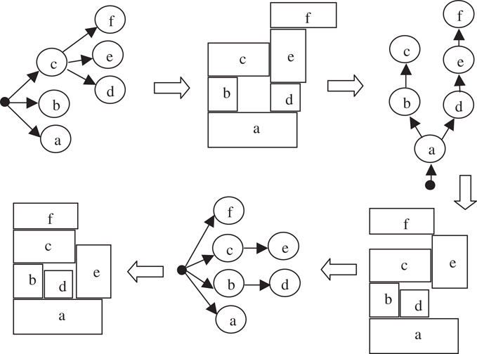
Figure 54.17Transformation between horizontal and vertical O-trees.
On the other hand, given an LB-compact floorplan, we can always derive an O-tree representation. For example, Figure 54.18 illustrates a general floorplan with seven blocks and the corresponding O-tree. O-tree is able to cover LB-compact floorplan with the smallest number of combinations in Table 54.1 and Figure 54.2 because the O-tree structure avoids redundancy and screens improper floorplans by taking advantage of the knowledge of the block dimensions. For example, given an O-tree, we can convert it to a binary tree and find many other possible trees to pair up as twin binary trees, which correspond to many different mosaic floorplans. In the perspective of O-tree representation, these floorplans are the variations due to the differences of the block sizes.
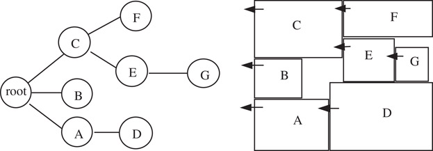
Figure 54.18An O-tree representation of a general floorplan.
The B* tree and the O-tree are equivalent because the transformation between the two is one to one mapping. The merit of the B tree is a different data structure and implementation.
In summary, among the constraint-graphs based representations, from the point of view of the pointers necessary for representing the floorplans, O-tree is a subset of twin binary tree; twin binary is a subset of corner stitching; and corner stitching is a subset of constraint graphs, as demonstrated in Figure 54.19.
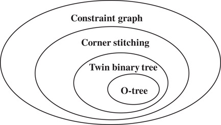
Figure 54.19Relationship between the constraint graph based representation.
54.3Placement Based Representations
The placement-based representations include sequence pair, bounded-sliceline grid, corner block list and slicing tree. With the dimensions of all the blocks known, the sequence pair and bounded-sliceline grid can be applied to general floorplans. The corner block list records the relative position of adjacent blocks, and is applicable to mosaic floorplan only. The slicing tree is for slicing floorplan, which is a special case of mosaic floorplan.
Sequence-pair expresses the topological positions of blocks with a pair of block lists [16,17]. For each pair of blocks, there are four possible relations, left-right, right-left, above-below, and below-above. We use a pair of sequences {π1, π2} to record the order of the two blocks. We can record two blocks A, B in four different orders: (AB, AB), (AB, BA), (BA, AB), (BA, BA). Hence, we use the four orders to represent the four placement relations. Figure 54.20 shows the four possible relations between a pair of blocks A and B and the corresponding sequence pair for each relation.
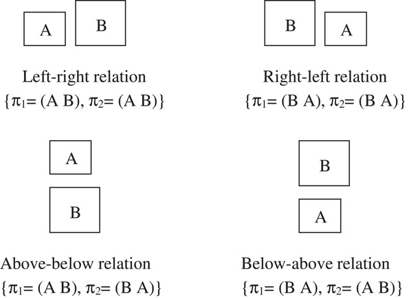
Figure 54.20Four possible relations between a pair of blocks.
The two sequences can be viewed as two coordinate systems that define a grid placement of the blocks. To see it more clearly, we construct a grid system illustrated in Figure 54.21. The slopes are denoted with the labels of blocks according to their orders in the two sequences. The intersections of two perpendicular lines that have the same label indicate the topological positions of the blocks.
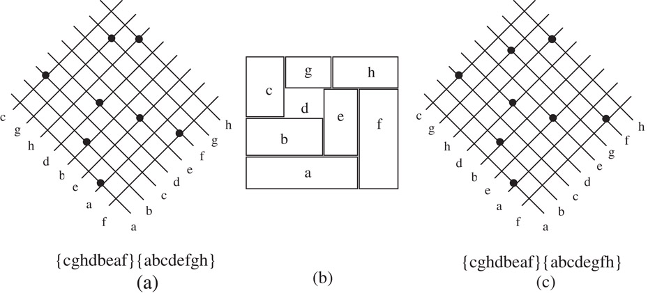
Figure 54.21The grid system and the redundancy.
The grid placement defines the floorplan relation between blocks. For each node in the grid placement, we divide the whole space into four quadrants, quadrant I: − 45 to 45°, quadrant II: 45–135, quadrant III: 135–225, quadrant IV: 225–315. Block B’s floorplan relation with block A can be derived from block B’s location in block A’s quadrants.
1.Quadrant I: block B is on the right of block A
2.Quadrant II: block B is above block A
3.Quadrant III: block B is on the left of block A
4.Quadrant IV: block B is below block A
For example, from the grid placement in Figure 54.22, using node d as a reference, blocks e and f are on the right of block d; blocks g and h are above; blocks c is on the left; and blocks a and b are below.

Figure 54.22Derivation of sequence-pair.
We can derive the sequence-pair from a floorplan by tracing the blocks through two directions. We first extend the boundary of each block by drawing lines from its four corners (Figure 54.22). In Figure 54.22a, we draw a line from the upper-right corner of each block that goes either rightward or upward. When the line is obstructed with a block or an already existing line, it changes its direction. The extension of the line ends when it reaches the boundary of the chip. We also draw a line from the lower-left corner of each block that goes either downwards or leftwards. The extended lines partition the chip into zones. Following the order of the zones, we get a label sequence. For instance, we have π1 = ′ecafdg′ for Figure 54.22a. With similar operations, the second sequence is derived in the orthogonal direction (π2 = ′fcegad′ in Figure 54.22b). π1 and π2 consist of a sequence-pair, which involves all the information of the topological positions of blocks.
For translating a sequence-pair into a topological floorplan with n blocks, a brute force implementation requires time complexity O(n2), since there are O(n2) pairs of blocks and we need to scan all the pairs to get the constraint graph and then derive the floorplan by performing a longest path computation. In Reference 3, a fast algorithm with O(nloglogn) time complexity is proposed to complete the transformation of a sequence pair to the floorplan. The fast algorithm takes advantage of the longest common sequence of the two sequences in a sequence-pair. They show that the longest common sequence calculation is equivalent to the longest path computation in the constraint graph for a sequence-pair. The authors use a priority queue data structure to record the longest common sequence, thus reduce the time for calculating the position of a single block to O(loglogn) by amortizing.
The representation of a sequence-pair has the following properties:
1.The number of bits for storing a sequence-pair is 2n log2n, where n is the number of blocks in the placement.
2.The time complexity of translating a sequence-pair into a topological floorplan is by the newest report.
3.There are totally (n!)2 possible sequence-pairs for n blocks. However, there exists the redundancy. For example, the sequence-pairs in Figure 54.21a and c actually correspond to the same placement (Figure 54.21b).
Another method rising from the same idea as sequence-pair is BSG [4], where, instead of the intersections of grid lines, the squares surrounded by the grid lines, called rooms, are used to assign the blocks (Figure 54.23). Although put forward aiming at the packing problem, BSG can also act as a compacting algorithm to determine the accurate positions of blocks.
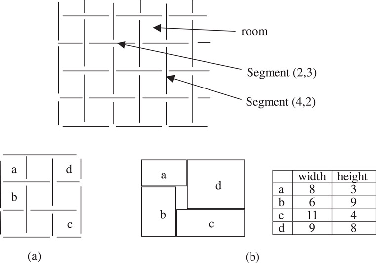
Figure 54.23Basic structure of BSG.
In BSG, grid lines are separated into vertical and horizontal segments (Figure 54.23). Two constraint graphs are set up with their vertexes corresponding to the grid segments and their directed edges corresponding to the relative positions of the grid segments (Figure 54.24). The vertexes “source” and “sink” are added to make the operation on the graph easy. Every room is crossed by one edge of the constraint graph (respectively in the vertical and horizontal constraint graphs). If the room is not empty, or there is a block assigned into the room, the crossing edge has a weight equal to the width (in the horizontal graph) or the height (in the vertical graph) of the assigned block, otherwise the crossing edge has a weight of zero. Figure 54.24 shows the weights derived from the example in Figure 54.23. By calculating the longest path lengths between the source and the other vertexes in the constraint graphs the real coordinates of the grid segments can be determined and in fact the translation to the placement is implemented. Table 54.4 gives the final results of the example in Figure 54.23 and Figure 54.24. Notice that segment (1, 3) and (2, 2) have the same position, for the edge between the two vertexes in the horizontal constraint graph has the weight of zero.
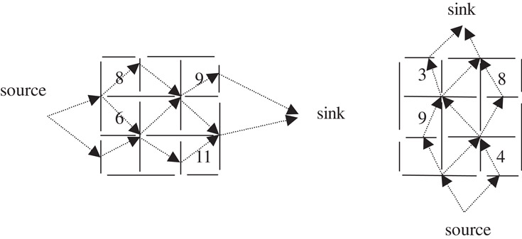
Figure 54.24Constraint graphs.
Table 54.4Physical Positions of Segments

Due to the homology, BSG has the similar performance as sequence-pair, except that the complexity of the translation into placement, or finding the longest path lengths for all the vertexes in the constraint graphs, is O(pq), provided that the grid array has p columns and q rows.
Corner block list is a third method of representing non-slicing structures [5,18,19]. Refer to Figure 54.25. The floorplan is required to be mosaic and without degeneration.
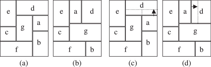
Figure 54.25Corner block list.
For every block, the T-junction at the bottom-left corner can be in either of the two directions. Accordingly we say the orientation of the block is 1 or 0 respectively. Now let’s observe the most upper-right blocks in Figure 54.25a and (b), both denoted with “d.” If we push the bottom boundary of block “d” in (a) upwards, or the left boundary in (b) rightwards, then block “d” is squeezed and finally deleted (Figure 54.25c and d), and thereafter block “a” becomes the most upper-right block. The operation of squeezing and deleting can be repeatedly performed until there is only one block left in the placement.
According to the order in which the blocks are squeezed out, we get two lists. The labels of blocks are stored in list “S” while the orientations of the blocks in list “L.” For example, for Figure 54.25a, S = “fcegbad” and L = “001100.” S and L are not sufficient to recover the placement, so we need the third list, T. Each time we squeeze a block, we record the number of T-junctions on the moving boundary, excluding the two at its ends, then add the same number of “1”s and one “0” into T. For example, in Figure 54.25a, when squeezing block d, we have T = “01,” for there is only one T-junction on the bottom boundary, which separates the blocks a, d and g. Next, while squeezing block a, only a “0” is added to T, for there is no T-junction on the bottom boundary of block a. Consequently, we have T = “001” after the deletion of block a, and T = “00101001” after the deletion of block c. With an inverse process, the placement can be recovered from S, L and T.
The performance of corner block list is:
1.The storage of the 3 lists needs at most n(3 + logn) bits.
2.The number of combinations is TRIALRESTRICTION, which is the same as that of a slicing tree. However, slicing structure only covers part of all possible combinations, therefore has larger redundancy than corner block list.
3.The complexity of the translation between placement and lists is TRIALRESTRICTION.
A floorplan is call a slicing structure [20,21] if it can be iteratively partitioned into two parts with vertical or horizontal cut lines throughout the separated parts of the area, until the individual blocks. Figure 54.26a gives an example. Line 1 splits the whole layout into two parts. The left half involves only one block but the right half can been further split by line 2. Then follows line 3, line 4, and so on. On the contrary, Figure 54.26b is a non-slicing structure. We can’t find a cut line throughout the floorplan to split it into two parts.
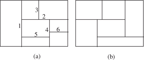
Figure 54.26Slicing structure and non-slicing structure.
Now that a slicing floorplan can been iteratively split into two parts with vertical or horizontal cut lines, a binary tree can be structured according to the splitting process [22].
Figure 54.27 gives an example of a slicing floorplan and its binary tree. The inter nodes on the tree denoted with “H” or “V” indicate the direction of the line splitting the areas, while the leaf nodes correspond to the blocks. We call the binary tree a slicing tree.
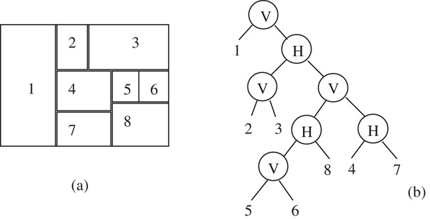
Figure 54.27Slicing structure and its binary tree representation.
Just as in twin binary tree, we hope to find a simple data structure to express the slicing tree. Polish Expression is a good solution. It is the result of a post-order traversal on the slicing tree. As an example, the Polish Expression of Figure 54.27 is: 123V56V8H47HVHV. We regard “H” and “V” as operators and the blocks operands.
Formally, we have the following definition for a Polish expression:
A sequence of elements from {1, 2, …, n, V, H} is a Polish expression of length 2n − 1 iff:
1.Every subscript i appears exactly once in the sequence, 1 ≤ i ≤ 2n − 1.
2.The number of operators is less than the number of the components for any prefix sub-string.
So needless to re-construct the slicing tree, we are able to judge a legal Polish Expression. For example, 21H57V43H6VHV and 215H7V43H6VHV are legal Polish Expressions while 215HVHV7436HV and 2H15437VVVHH are not. An illegal Polish Expression can’t be converted to a binary tree.
It is obvious that for a given slicing tree, we have a unique Polish Expression. Inversely, we can easily conduct the slicing tree according to its Polish Expression. So we conclude that there is a one-to-one correspondence between the slicing tree and Polish Expression. However, there may be more than one slicing tree corresponding to one floorplan, as shown in Figure 54.28. Thus there exists redundancy. To compact the solution space, we define the skewed slicing tree to be a slicing tree without a node that has the same operator as its right son. Correspondingly, a normalized Polish expression is defined:
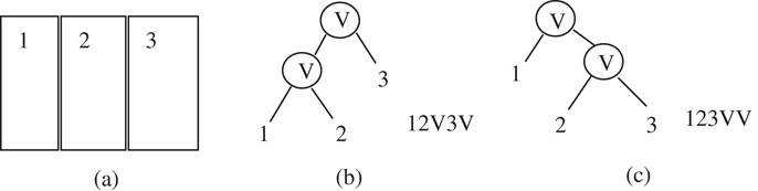
Figure 54.28Redundancy of slicing trees.
A Polish expression is called to be normalized iff there is no consecutive “V” or “H” in the sequence.
In Figure 54.28, (b) is a normalized Polish expression while (c) is not. There is a one-to-one correspondence between the set of normalized Polish expressions and the set of slicing structures.
To perturb the blocks to get new solutions, we define three types of perturbations on polish expressions:
M1: Swap two adjacent operands. For example, 12V3H →13V2H;
M2: Complement some chain of operators. For example, 12V3H→12V3V;
M3: Swap two adjacent operand and operator. For example, 12V3H→123VH;
The operation of M3 may result in a non-normalized Polish Expression. So a check is necessary after an operation of M3 to guarantee that a normalized expression is generated.
Figure 54.29 illustrates two sequences of polish expression transformations as well as their corresponding floorplans. We can see that a slight modification on the Polish Expression can result in a completely different floorplan topology. This is just what we want.
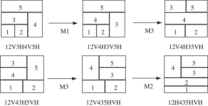
Figure 54.29Slicing structure moves.
Finally, we analyze the performance of slicing tree.
1.Given a floorplan of n blocks, the slicing tree contains n leaves and n − 1 internal nodes.
2.The number of possible configurations for the tree is .
3.The storage of a Polish Expression needs a 3n-bit stream plus a permutation of n blocks.
4.It will take linear time to transform a floorplan into a slicing tree, and vice versa.
54.4Relationships of the Representations
We summarize the relationships between the representations in this section. A mosaic floorplan example and a general floorplan example are also discussed in detail to show the relationships.
54.4.1Summary of the Relationships
According to the definitions of the representations, we have four relationships between the sequence-pair (SP), the corner block list (CBL), the twin binary tree (TBT) and the O-Tree representations.
For further discussions, we first define the 90° rotation of a floorplan as follows:
Definition 90° rotation of a floorplan: We use F90 to denote the floorplan obtained by rotating floorplan F, 90 degrees counterclockwise.
The four relationships are as follows and summarized in Figure. 54.30.
1.Given a mosaic floorplan and its corresponding corner block list CB = (S, L, T), there exists a sequence pair SP = (S1, S2) corresponding to the same floorplan such that the second sequence of SP is same as the sequence S of the corner block list.
2.Given a mosaic floorplan and its corresponding twin binary trees (), there exists a sequence pair corresponding to the same floorplan such that the first sequence of SP is the same as the node sequence of in-order traversal in tree τ+.
3.Given a mosaic floorplan and its corresponding twin binary trees , there exists an O-tree corresponding to the same floorplan such that τ− is identical to the O-tree after the tree conversion from a binary tree to an ordered tree.
4.Given a mosaic floorplan F, and its corresponding twin binary trees , the node sequence of in-order traversal in tree τ+ is identical to the sequence S in the corner block list CB = (S, L, T) of the floorplan F90.
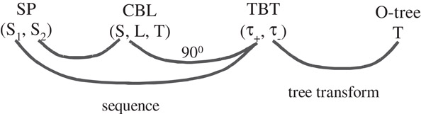
Figure 54.30Summary of the relationships between floorplan representations.
54.4.2A Mosaic Floorplan Example
Figure 54.31 describes an example of a mosaic floorplan. We illustrate the four representations. The twin binary trees are marked with circles and crosses as shown in Figure 54.31. Two SPs, SP1 and SP2, out of many possible choices, are described in the figure.
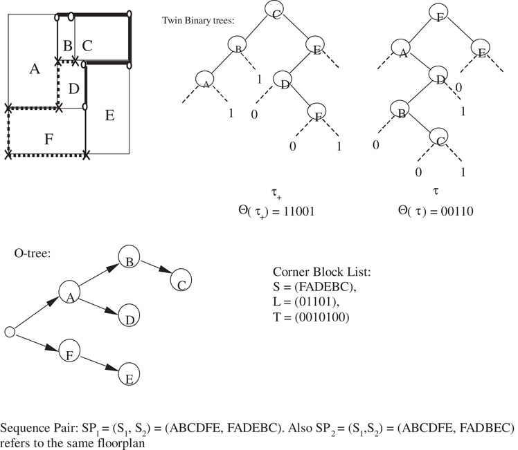
Figure 54.31A mosaic floorplan and its different representations.
The in-order traversal of the τ+ in the twin binary trees representation produces the sequence π(τ+) = ABCDFE, which is same as the first sequence of SP1 and SP2. In Figure 54.31, an O-tree representation is also given. Its binary tree representation is identical to the τ− of the twin binary trees after tree conversion. The corner block list representation is next to the O-tree representation in Figure 54.31. Its sequence S = FADEBC is same as the second sequence of SP1.
Figure 54.32 shows the 90° rotation of the mosaic floorplan in Figure 54.31. The CB (S,L,T) representation of F90 has S = ABCDFE (Figure 54.32.), which is identical to π(τ), the order of the twin binary trees representation () of the floorplan in Figure 54.31.
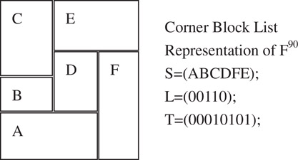
Figure 54.3290° rotation of the floorplan in Figure 54.31.
54.4.3A General Floorplan Example
Figure 54.33 illustrates a general floorplan. Only the O-tree and the sequence pair are capable of representing this general floorplan. The O-tree and SP representations are shown in the figure.
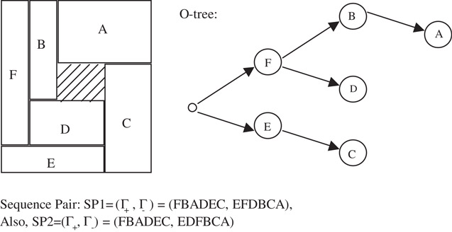
Figure 54.33A general floorplan with its O-tree and SP representation.
54.5Rectilinear Shape Handling
Shape handling makes feasible the treating of blocks with arbitrary shapes. It makes sense especially in deep sub-micron technology, where, with the number of routing layers increasing, wires are placed in layers other than the device layer, and the placement becomes more like a packing problem: a set of macro blocks are packed together without overlaps, with some objective functions minimized.
The basic idea to handle the arbitrary-shaped blocks is to partition them into rectangles, and then the representations and the optimizing strategies described above can be used. Figure 54.34a and b demonstrate two schemes of partitioning, the horizontal one and the vertical one. However, if the generated rectangle blocks were treated as individual ones, it would be quite impossible to recover the original blocks. The generated rectangle blocks may be shifted (Figure 54.34c) or separated (Figure 54.34d). So extra constraints have to be imposed on the generated rectangle blocks in order to keep the original blocks’ shapes.
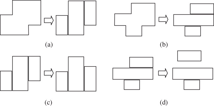
Figure 54.34Shape handling.
One proposed method of adding extra constraints is illustrated with Figure 54.35b for horizontal and (c) for vertical. The vertexes in the constraint graph correspond to the generated rectangle blocks, while the direct edges denote the relative positions of the blocks. For example, an edge from “a” to “b” with a weight of 1 means that block “b” lies to the right of “a,” the distance between their left boundaries is 1, which is exactly the width of “a.” Because the relative-position constraints are always represented with the format such as “larger than or equal to” during optimization, inversely directed edges, such as the edge from “b” to “a” with a negative weight, helps to determine the position relationships solely.
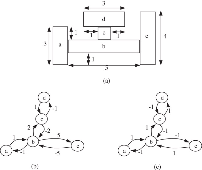
Figure 54.35An example of adding extra constraints.
Floorplan representation is an important issue for floorplan optimization. We classify the representations into graph based and placement based methods based on the different strategies used in deriving the representations. The graph-based methods are based on the constraint graphs, which include the constraint graphs, the corner stitching, the twin binary tree and the O-tree. The placement-based methods are based on the local topology relations in deriving the floorplans, which include the sequence pair, the bounded sliceline grid, the corner block list and the slicing tree.
The floorplans can also be classified into different categories: general, mosaic and slicing floorplans. Slicing floorplan is a subset of mosaic floorplan, which is again a subset of the general floorplan. We have different representations for different types of floorplans. The constraint graphs, the corner stitching, the sequence pair, the bounded sliceline grid and the O-trees are for general floorplans. The twin binary tree and the corner block list are for mosaic floorplans. The slicing tree is for slicing floorplans. Different representations have different solution spaces and time complexities to derive a floorplan.
The authors are grateful to Mr. Simon Chu of Sun Microsystems for his thorough review of the chapter.
1.W. Dai and E.S. Kuh, “Hierarchical Floor Planning for Building Block Layout,” in IEEE Int. Conf. on Computer-Aided Design, 1986, pp. 454–457.
2.B. Yao, H. Chen, C.K. Cheng, and R. Graham, “Revisiting Floorplan Representations,” in Proc. International Symposium on Physical Design, 2001, pp. 138–143.
3.X. Tang and M. Wong, “FAST-SP A Fast Algorithm for Block Placement Based on Sequence Pair,” in Proc. of Asia and South Pacific Design Automation Conference, pp. 521–526, Yokohama, Japan, Jan. 2001.
4.S. Nakatake, K. Fujiyoshi, H. Murata, and Y. Kajitani, “Module Packing Based on the BSG-Structure and IC Layout Applications,” IEEE Trans. on Computer-Aided Design of Integrated Circuits and Systems, vol. 17, no. 6, June 1998, pp. 519–530.
5.X. Hong, G. Huang, Y. Cai, J. Gu, S. Dong, C.K. Cheng, and J. Gu, “Conner Block List: An Effective and Efficient Topological Representation of Non-Slicing Floorplan,” in Proceeding of ICCAD-2000, 2000, pp. 8–12.
6.M. Abe, “Covering the Square by Squares without Overlapping (in Japanese),” J. Japan Math. Phys., vol. 4, no. 4, 1930, pp. 359–366.
7.K. Sakanushi, Y. Kajitani, and D.P. Mehta, “The Quarter-State-Sequence Floorplan Representation,” IEEE Trans. on Circuits and Systems—I, vol. 50, no. 3, 2003, pp. 376–385.
8.F.Y. Young, C.N. Chu, and Z.C. Shen, “Twin Binary Sequences: A Non-Redundant Representation for General Non-Slicing Floorplan,” in Proc International Symposium on Physical Design, 2002, pp. 196–201.
9.K. Kozminsky and E. Kinnen, “Rectangular Duals of Planar Graph,” Networks, vol. 15, 1985, pp. 145–157.
10.R.L. Brooks, C.A.B. Smith, A.H. Stone, and W.T. Tutte, “The Dissection of Rectangle into Squares,” Duke Math, Journal, vol. 7, 1940, pp. 312–340.
11.J.M. Lin and Y.W. Chang, “TCG: A Transitive Closure Graph-Based Representation for Non-Slicing Floorplans,” in Proc: DAC, 2001, pp. 764–76.
12.J. Ousterhoust, “Corner Stitching: A Data-Structuring Technique for VLSI Layout Tools,” in IEEE Transactions on Computer-Aided Design, CAD-3, January 1984, pp. 87–100.
13.P. Guo, C.K. Cheng, and T. Yoshimura, “An O-Tree Representation of Non-Slicing Floorplan and Its Applications,” in Proc: 36th DAC, 1999, pp. 268–273.
14.Y. Pang, C.K. Cheng, K. Lampaert, and W. Xie, “Rectilinear Block Packing Using O-Tree Representation,” in Proc. ISPD, 2001, pp. 156–161.
15.Y. Chang, G. Wu, and S. Wu, “B*-Trees: A New Representation for Non-Slicing Floorplans,” in Proc. 37th DAC, 2000, pp. 458–463.
16.H. Murata, K. Fujiyoushi, S. Nakatake, and Y. Kajitani, “Rectangle-Packing-Based Module Placement,” in Proc. of International Conference on Computer Aided Design, 1995, pp. 472–479.
17.J. Xu, P. Guo, and C.K. Cheng, “Sequence-Pair Approach for Rectilinear Module Placement,” in IEEE Trans. on CAD, April 1999, pp. 484–493.
18.S. Zhou, S. Dong, X. Hong, Y. Cai, J. Gu, and C.K. Cheng, “ECBL: An Extended Corner Block List with O(n) Complexity and Solution Space Including Optimum Placement,” in Int: Symp. on Physical Design, 2001, pp. 150–155.
19.Y. Ma, X. Hong, S. Dong, Y. Cai, C.K. Cheng, and J. Gu, “Floorplanning with Abutment Constraints and L-Shaped /T-Shaped Blocks Based on Corner Block List,” in ACM/IEEE Design Automation Conf., 2001, pp. 770–775.
20.R.H.J.M. Otten, “Automatic Floorplan Design,” in Proc. ACM/IEEE Design Automation Conf., 1982, pp. 261–267.
21.D.F. Wong and C.L. Liu, “A New Algorithm for Floorplan Design,” in ACM/IEEE Design Automation Conf., 1986, pp. 101–107.
22.A.A. Szepieniec and R.H.J.M. Otten, “The Genealogical Approach to the Layout Problem,” in Proc. of the 17th Design Automation Conference, 1980, pp. 535–542.
23.D.E. Knuth, The Art of Computer Programming, Addison-Wesley Press, 1997.
24.R.H.J.M. Otten, “What is a Floorplan,” in Proc. of International Symposium on Physical Design, 2000, pp. 212–217.
25.J. Grason, A Dual Linear Graph Representation for Space-filling Location Problems of the Floor-planning Type, MIT Press, Cambridge (Mass), USA, 1970.
26.K. Sakanushi and Y. Kajitani, “The Quarter-State Sequence (Q-Sequence) to Represent the Floorplan and Applications to Layout Optimization,” in Proc. IEEE APCCAS, 2000, pp. 829–832.
27.J. Xu, P. Guo, and C.K. Cheng, “Cluster Refinement for Block Placement,” in Proc. ACM/IEEE Design Automation Conf., 1997, pp. 762–765.
28.J. Xu, P. Guo, and C.K. Cheng, “Empirical Study of Block Placement by Cluster Refinement,” VLSI Design, vol. 10, no. 1, pp. 71–86, 1999.
29.C. Zhuang, K. Sakanushi, J. Liyan, and Y. Kajitani, “An Enhanced Q-Sequence Augmented with Empty-Room-Insertion and Parenthesis Trees,” in Design Automation and Test in Europe Conference and Exhibition, 2002, pp. 61–68.
*This chapter has been reprinted from first edition of this Handbook, without any content updates.