
Dale McMullin †
Colorado School of Mines
Alyn Rockwood †
Colorado School of Mines
Meshes•CAD/CAM Drawings•Fonts•Bitmaps•Texture Mapping
Vertices, Edges, and Faces•Vertex, Normal, and Face Lists•Winged Edge•Tiled,Multidimensional Array•Linear Interpolation and Bezier Curves
55.4Applications of Previously Discussed Structures
Hidden Surface Removal: An Application of the BSP Tree•Proximity and Collision: Other Applications of the BSP Tree•More With Trees: CSG Modeling
Like all major applications within the vast arenas of computer science and technology, the computer graphics industry depends on the efficient synergy of hardware and software to deliver to the growing demands of computer users. From computer gaming to engineering to medicine, computer graphics applications are pervasive. As hardware capabilities grow, the potential for new feasible uses for computer graphics emerge.
In recent years, the exponential growth of chipset speeds and memory capacities in personal computers have made commonplace the applications that were once only available to individuals and companies with specialized graphical needs. One excellent example is flight simulators. As recently as twenty years ago, an aviation company would have purchased a flight simulator, capable of rendering one thousand shaded polygons per second, for ten million dollars. Even with a room full of processing hardware and rendering equipment, it would be primitive by today’s graphics standards. With today’s graphics cards and software, one renders tens of millions of shaded polygons every second for two hundred dollars.
As the needs for graphics applications grow and change, research takes the industry in many different directions. However, even though the applications may evolve, what happens under the scenes is much more static; the way graphics primitives are represented, or stored in computer memory, have stayed relatively constant. This can be mainly attributed to the continued use of many standard, stable data structures, algorithms, and models. As this chapter will illustrate, data and algorithmic standards familiar to computer science lend themselves quite well to turning the mathematics and geometries of computer graphics into impressive images.
Graphics hardware plays an important role in nearly all applications of computer graphics. The ability for systems to map 3–D vertices to 2–D locations on a monitor screen is critical. Once the object or “model” is interpreted by the CPU, the hardware draws and shades the object according to a user’s viewpoint. The “pipeline” [1], or order in which the computer turns mathematical expressions into a graphics scene, governs this process. Several complex sub-processes define the pipeline. Figure 55.1 illustrates a typical example.
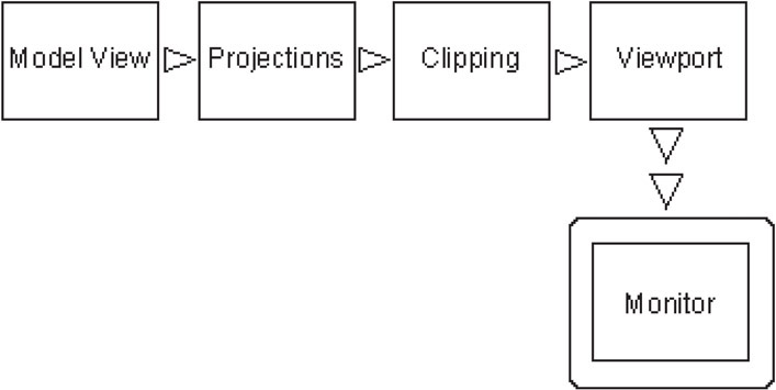
Figure 55.1Graphics pipeline.
The Model View is the point where the models are created, constructed as a combination of meshes and mapped textures. The Projection point is where the models are transformed (scaled, rotated, and moved) through a series of affine transformations to their final position. Clipping involves invoking algorithms to determine perspective, and what objects are visible in the Viewport. The Viewport readies the scene for display on the computer’s monitor. The final scene is “rasterized” to the monitor [1].
Standard data structures and algorithms apply to all steps in the pipeline process. Since the speed of most rendering hardware (and hence the pipeline) is directly dependent on the number of models to be drawn, it becomes important to utilize structures that are as efficient as possible. In fact, graphics hardware is often designed and engineered to cater to a specific, standard form of data representation.
In both 2-D and 3-D applications, objects are modeled with polygons and polygon meshes. The basic elements of a polygon mesh include the vertex, the edge, and the face. An edge is composed of the line segment between two vertices, and a face is defined by the closed polygon of three or more edges. A mesh is formed when two or more faces are connected by shared vertices and edges. A typical polygon (triangle) mesh is shown in Figure 55.2.
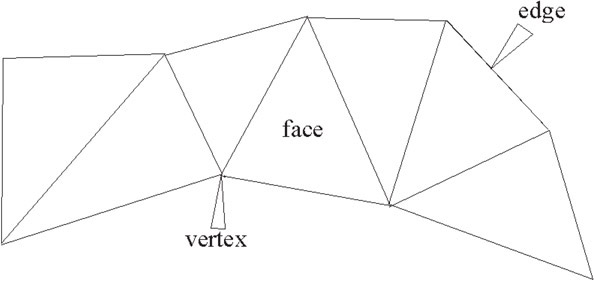
Figure 55.2A triangle mesh.
Specific examples of meshes include “triangle meshes, polygon meshes, and polygon meshes with holes.” [2] However, the triangle is currently the most popular face geometry in standard meshes. This is mainly because of its simplicity, direct application to trigonometric calculations, and ease of mesh storage (as we will see).
In Computer Aided Design (CAD), Computer Aided Manufacturing (CAM), and other channels of engineering design, we see the same basic elements. During the design process of everything from automobiles to telephones, applications are used to “see” the parts before they are manufactured. The physical interactions and assemblies of parts can be tested before any steel is milled or plastic is poured.
Figure 55.3 illustrates a wire-frame (and fully rendered) model of a drill bit used in the oil and gas industry. Every modeled element of this design requires a definition of vertices and edges. These vertices define single-line edges, polyline edges, and the curved edges. The proximity of vertices to edges, edges to edges, and vertices to vertices may be tested for tolerances and potential problems. The software makes the stored model visible to the user within the current coordinate system and viewpoint. It is then up to the user to interface the visual medium with his or her engineering (or design) training to create a useful design.
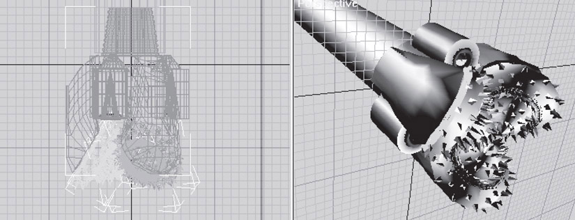
Figure 55.3Models of a drill bit.
Even in wire frame models, we see the application of more sophisticated graphics practices. Note how many of the contours of the drill bit parts are not connected line segments, but actual smooth curves. This is an example of where vertices have been used not to define edges, but the “control points” of a Bezier Curve. How curves like the B-Spline and Bezier utilize vertices in their structures is discussed later in this chapter. For now it is sufficient to mention that these types of curves are present in nearly all corners of the graphics industry.
Fonts are another example of where the vertex is used, in two dimensions, as the basis of a data structure in order to define the appearance of each character and number in various languages. Several examples of interesting Greek characters, each defined by a different font definition file, and at different sizes, are shown in Figure 55.4.
![]()
Figure 55.4Fonts.
The typical Postscript font is defined by a number of points, read in as control points for each curve (or line) in the font character. The “Postscript” driver software is then used to interpret the control points and render the characters with Bezier curves (see Section 55.3.5).
Perhaps the most important concept is that each pixel of the font character does not have to be stored, only a small number of vertex definitions. As the control points are transformed through operations like italicizing, the curves remain aligned in the proper proportion to the original character. Note the “M” character in the above figure has been italicized. The “Postscript” font representation serves as a very effective example of how a single standardized data structure of specific size can be utilized to define a potentially infinite number of characters.
Bitmaps are a cornerstone to computer graphics. In fact, the name “bitmap” has become a commodity to most computer users in the way that it describes a computer generated picture. A bitmap is a very simple, yet versatile, way to store a graphic image as a binary file. The file header structure of a bitmap [3] in itself is a standard data structure, as the following illustrates:
 struct _BITMAP
 {
 Uint8 bmType;
 Uint8 bmBitsPerPixel;
 Uint8 bmBytesPerPixel;
 Uint8 bmReserved;

 Uint32 bmColorKey;

 Uint32 bmWidth;
 Uint32 bmHeight;
 Uint32 bmPitch;

 void* bmBits;
 };
The bitmap is initially defined by a number of parameters that define the type, width, height, etc. of the graphic image. These properties are stored in the header of the file as shown. The actual “pixels” required to fill that space is then defined in the “bmBits” pointer. As a rule, the total number of pixels in the image memory will equal the width times the height divided by the “bits per pixel” property. The “bytes per pixel” property determines how the “bits per pixel” are divided among the individual color components of each pixel. For instance, a bitmap with RGB color map is commonly defined by twenty four (24) bits per pixel and three (3) bytes per pixel. Each of the three bytes for each pixel use 8 of the twenty four bits to define red, green, and blue values respectively.
Early bitmaps, when color monitors were first being used, were defined with 4-bit color. In other words, each color was defined by a 4-bit (or half-byte) word. Since a half-byte has a maximum value of 24 or 16, 4-bit bitmaps were capable of supporting sixteen (16) different colors. The required disk space to store a 100 × 100 4-bit bitmap would then be 10,000* .5 bytes or 5,000 Bytes (5kB).
In the past fifteen years, the need for more realistic graphics has driven the increase in the memory used for color. Today 24-bit (also called true color) and 32-bit color, which both represent 16.7 million colors (32-bit adds an extra byte for the alpha channel), are the most commonly supported formats in today’s hardware. The alpha channel refers to a single byte used to store the transparency of the color. Bitmap files in these formats now require 3 and 4 bytes per pixel. Additionally, current monitor resolutions require over 1,000 pixels in width or height, and thus graphic files are growing even larger. Figure 55.5 is a photograph that has been scanned in and stored as a bitmap file.
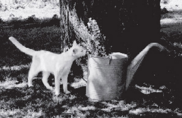
Figure 55.5Bitmap file.
A typical 5 × 7 photograph, at 100 dpi (dots per inch), and 24-bit color, would require 500 × 700 × 3 or 1.05 megabytes (MB) to store in a conventional bitmap format. Because of the increased size requirements in bitmaps, compression algorithms have become common-place. File formats such as JPG (jpeg) and PNG (ping) are examples of widely used formats. However, there is a tradeoff. When a compression algorithm is applied to a bitmap, a degree of image quality is inevitably lost. Consequently, in applications like publishing and graphic art, uncompressed bitmaps are still required where high image quality is expected.
The processes of texture and surface mapping represent an application where bitmaps and polygonal meshes are combined to create more realistic models. Texture mapping has become a cornerstone of graphics applications in recent years because of its versatility, ease of implementation, and speed in graphical environments with a high number of objects and polygons. In fact, today’s graphics hardware ships with the tools necessary to implement the texture and surface mapping processes on the local chipset, and the data structures used in rendering environments are largely standardized.
Prior to texture mapping, 3-D polygonal meshes were processed through shading models such as Gouraud and Phong to provide realism. Each shading model provides the means for providing color, shadows, and even reflection (glare) to individual components of the model. This was accomplished through a mathematical model of how light behaves within specular, diffuse, reflective, and refractive contexts. The general shading equation for light intensity, I, based on the individual ambient, diffuse, and specular components is shown below.
where
![]()
![]()
![]()
![]()
![]()
The primary difference between Gouraud and Phong is in that Phong provides the additional component for specular reflection, which gives objects a more realistic glare when desired. Also, because the Phong model requires more detail, the intensity values are calculated (interpolated) at each pixel rather than each polygon. The vectors m, s, and h represent the normal, reflected, and diffuse light from a given polygonal surface (or face). Linear interpolation, a widely used algorithm in graphics, is discussed in Section 55.3.5.
Although still used today, these shading models have limitations when more realistic results are desired. Because color and light reflection are modeled on individual model components, the model would have to be constructed as a composite of many different components, each with different color (or material) properties, in order to achieve a more realistic effect. This requires models to be much more complex, and increasingly difficult to construct. If changes in surface appearance or continuity were desired, they would have to be physically modeled in the mesh itself in order to be viewed.
Texture and surface mapping have provided a practical solution to these model complexity dilemmas. The mapping methods involve taking the input from a bitmap file, like those described previously, and “stretching” them over a polygonal mesh. The end result is a meshed object.which takes on the texture properties (or appearance) of the bitmap. The figure below illustrates a simple example of how the mesh and bitmap can be combined to create a more interesting object. Figure 55.6 shows how how Figure 55.5 has been “mapped” onto a sphere.
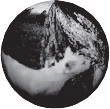
Figure 55.6Combination of mesh and bitmap.
The object seems to take on a more realistic appearance even when modeled by a very simple polygonal mesh. This technology has made fast rendering of realistic environments much more feasible, especially in computer games.
Texture, or “bump,” mapping utilizes a similar process as surface mapping, where a bitmap is stretched over a polygonal mesh. However, the pixels, commonly called “texels” [1], are used to alter how the light intensity interacts with the surface. Initially, the lighting model shown above would calculate an intensity, I, for a given surface. With texture mapping, individual grayscale values at each texel are used to alter the intensity vectors across each polygon in order to produce roughness effects.
Figure 55.7 illustrates a model of a sphere that has been rendered with the traditional Gouraud model, then Phong, and then finally rendered again with a texture map. This approach to improving model realism through mapping applies also to reflection, light intensity, and others.
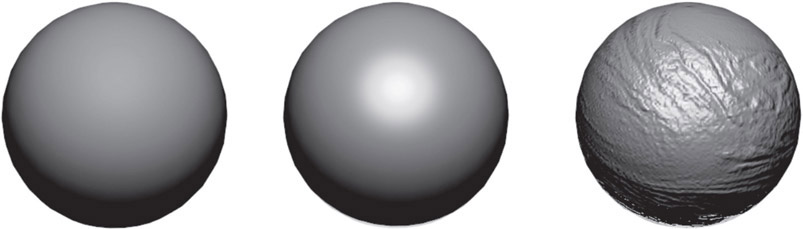
Figure 55.7Texture mapping.
55.3.1Vertices, Edges, and Faces
As mentioned previously, vertices, edges, and faces form the most basic elements of all polygonal representations in computer graphics. The simplest point can be represented in Cartesian coordinates in two (2D) and three dimensions (3D) as (x, y) and (x, y, z) respectively (Figure 55.8).

Figure 55.8Vertices, edges, and faces.
As a simple data structure, each vertex may then be stored as a two or three-dimensional array. Edges may then be represented by two-dimensional arrays containing the indexes of two points. Further, a face may be dimensioned based on the number of desired sides per face, and contain the indices of those edges. At first, this approach may seem acceptable, and in basic applications it is common to model each vertex, edge, and face as a separate class. Relative relationships between classes are then governed by the software to build meshes. However, modeling objects in this manner does have disadvantages.
Firstly, important information becomes difficult to track, such as the normal at each vertex, adjacency of faces, and other properties required for blending and achieving realism. Furthermore, the number of intersecting edges at each vertex may vary throughout the model, and mesh sizes between objects may be unpredictable. The ability to manage this approach then becomes increasingly difficult, with the potential for unnecessary overhead and housekeeping of relationships within the model. It then becomes necessary to create higher level data structures that go beyond these basic elements, and provide the elements necessary for efficient graphics applications.
55.3.2Vertex, Normal, and Face Lists
In this storage method, list structures are used to store three, inter-dependent lists of data. The first list defines the vertexes contained in the scene as follows. Each vertex is assigned an index, and a coordinate location, or (x, y, z) point. The second list defines the normals for each vertex. Again, each normal is assigned a numbered index and a 3-D coordinate point. The final list serves to integrate the first two. Each face is identified by a numbered index, an array of vertex indexes, and an array of indexed normals for each vertex. Figure 55.9 illustrates typical examples of a similar application with vertex, face, and edge lists.
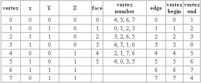
Figure 55.9Example of vertex, normal, and face lists.
In the table, three specific lists are evident. The first list represents each vertex in the model as it is defined in 3D space. The “vertex” column defines the id, index, or label of the vertex. The x, y, and z coordinates are then defined in the adjacent columns.
In the second list, six faces are defined. Each face has a label or index similar to the vertex list. However, rather than specifying coordinates in space, the adjacent column stores the id’s of the vertexes that enclose the face. Note that each face consists of four vertices, indicating that the each face will be defined by a quadrilateral.
The final list defines edges. Again, each edge definition contains a label or index column, followed by two adjacent vertex columns. The vertices of each edge define the start point and end point of each edge. In many applications of graphics, it is important to define the direction of an edge. In right handed coordinate systems, the direction of an edge will determine the direction of the normal vector which is orthogonal to the face surrounded by the edges.
Although one of the oldest data structures relating to polygonal structures, the Winged Edge approach is very effective, and still widely used [4]. This structure is different from the wireframe model in that edges are the primary focal point of organization.
In the structure, each edge is stored in an indexed array, with its vertices, adjacent faces, previous, and successive edges. This allows the critical information for each edge to be stored in an array of eight integer indexes; it is both consistent and scalable between applications. The structure is
Figure 55.11 illustrates a typical layout for a winged edge.
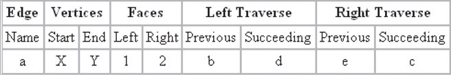
Figure 55.10Winged edge table.
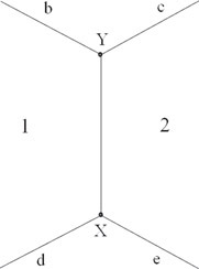
Figure 55.11Winged edge.
An important aspect of the Winged Edge structure is the order in which entries are listed. The edge itself has a direction, from the start vertex to the end vertex. The other entries are then defined by their proximity to the edge. If the direction of the edge were reversed, the right and left faces would change accordingly, as would the previous and succeeding entries of both the left and right traverse.
There is a time/space trade-off in using this model. What is saved in storage space adds to the needed time to find previous and successive edges. See Chapter 18 for more details.
55.3.4Tiled, Multidimensional Array
In this section we will discuss a data structure that is important to most geometric implementations. In many ways, the tiled array behaves identically to matrix data structures. For instance, a p by q matrix is normally stored as a single dimension array. However, since the matrix has p-rows and q-columns, the array needs to be addressed by creating an “offset” of size q in order to traverse each row. The following example should illustrate this concept.
Consider a matrix with p = 3 rows and q = 3 columns:
is stored as:
This represents where a 3 × 3 matrix is stored as an array with (3)(3) = 9 entries. In order to find the entry at row(i) = 3 and column(j) = 2 we employ the following method on the array:
Or in this case, Entry = A[2 + (3 − 1)(3)] = A[8] = 9
We use a similar method for tiling a single bitmap into several smaller images. This is analogous to each number entry in the above array being replaced by a bitmap with n by n pixels.
“Utilizing cache hierarchy is a crucial task in designing algorithms for modern architectures.” [1] In other words, tiling is a crucial step to ensuring multi-dimensional arrays are stored in an efficient, useful manner. Indexing mechanisms are used to locate data in each dimension. For example, a p by q array is stored in a one-dimensional array of length p * q, and indexed in row-column fashion as above.
When we wish to tile a p by q matrix into n by n tiles, the number of blocks in x is defined by q/n and the number of blocks in y is defined by p/n. Therefore, to find the “tile index” or the row and column of the tile for a value (x, y) we first calculate the tile location, or bitmap within the matrix of bitmaps. Then once the bitmap is located, the pixel location within that bitmap tile is found (sub-indexed). The entire two-step process can be simplified into a single equation that is executed once. Figure 55.12 illustrates this concept.
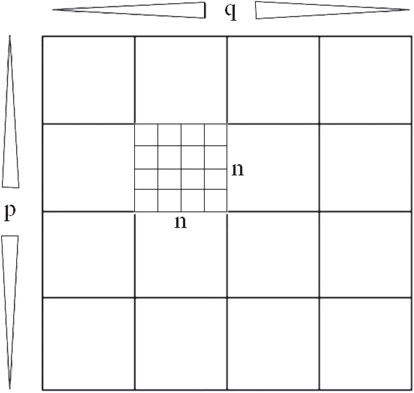
Figure 55.12Tiled array.
The final formula for locating x, y in a p by q array divided into n, n tiles is:
When dealing with matrices and combining multiple bitmaps and/or data into a Tile Multidimensional Array, performance and speed can both improve substantially.
55.3.5Linear Interpolation and Bezier Curves
This section will introduce one of the most significant contributions to design and graphics: the interpolated curve structure.
Linear interpolation refers to the parameterization of a straight line as a function of t, or:
where a, b are points in space. This equation represents both an affine invariant and barycentric combination of the points a and b. Affine invariance means that the point L(t) will always be collinear with the straight line through the point set {a, b}, regardless of the positioning of a and b. Describing this set as barycentric simply means that for t values between 0 and 1, L(t) will always occur between a and b. Another accurate description is that the equation L(t) is a linear “mapping” of t into some arbitrary region of space. Figure 55.13 illustrates this concept.
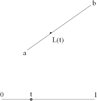
Figure 55.13Linear interpolation.
Linear interpolation is an extremely powerful concept. It is not only the foundation of many curve approximation algorithms, but the method is also used in many non-geometric applications as well, including calculating individual pixel intensities in the Phong shading method mentioned previously.
The basic Bezier curve derivation is based on an expanded form of linear interpolation. This concept uses the parameterization of t to represent two connected lines. The curve is then derived by performing a linear interpolation between the points interpolated on each line; a sort of linear interpolation in n parts, where n is the number of control points. The following example should illustrate:
Given are three points in space, {a, b, c}. These three points form the two line segments ab and bc (Figure 55.14).
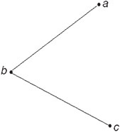
Figure 55.14Expanded form of linear interpolation.
During the first “iteration” of the Bezier curve derivation, linear interpolation is performed on each line segment for a given t value. These points are then connected by an additional line segment. The resulting equations (illustrated in Figure 55.15) are:
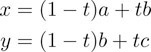
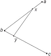
Figure 55.15First iteration of Bezier curve derivation.
The linear interpolation is performed one last time, with the same t value between the new points {x, y} (Figure 55.16):
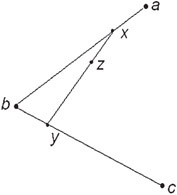
Figure 55.16Result of three linear interpolations.
This final point z, after three linear interpolations, is on the curve. Following this 3-step process for several “stepped” values for t between 0 and 1 would result in a smooth curve of z-values from a to c, and is illustrated in Figure 55.17:
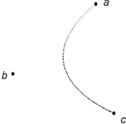
Figure 55.17Smooth curve.
This is a quadratic Bezier curve, and is represented mathematically by a linear interpolation between each set of x and y points, which were also derived through linear interpolation, for every t. By substituting the equations for x and y into the basic form, we obtain:
Simplified, we obtain a quadratic polynomial for a, b, and c as a function of the parameter t, or
The “string art” algorithm described previously is also referred to as the de Causteljau algorithm. Programmatically, the algorithm performs an n-step process for each value of t, where n is the number of “control points” in the curve. In this example, {a, b, c} are the control points of the curve.
Because of their ease of implementation and versatility, Bezier curves are invaluable in CAD, CAM, and graphic design. Also, Bezier curves require only a small number of control points for an accurate definition, so the data structure is ideal for compact storage. As mentioned previously, the Bezier form is the foundation for the Postscript font definition structure.
However, the Bezier form has limitations. When several attached curves are required in a design component, it takes considerable effort, or pre-calculation, to ensure the connected curves are “fair” or continuous with each other. Merely joining the end points of the curves may not be enough, resulting in “kinks” and other undesirable effects. For this reason, the B-spline curve provides an alternative to the Bezier where continuity is important. In fact, B-spline curves have often been referred to as a “user interface” for the Bezier form.
The goal of this section was to illustrate the versatility of linear interpolation and basic iteration structures in graphics and design. If more information is desired, numerous texts are currently available which describe the properties, mathematics, and applications of Bezier and B-spline curves, including the references listed at the end of this chapter.
55.4Applications of Previously Discussed Structures
55.4.1Hidden Surface Removal: An Application of the BSP Tree
In addition to other algorithms, BSP (Binary Space Partitioning) trees are one example where a specific, widely used, data structure has direct application in computer graphics. Hidden surface removal is essential to realistic 3-D graphics, and a primary application of BSP trees.
Hidden surface removal is used anywhere 3-dimensional objects must be made visible from multiple, if not infinite view points within a graphics scene. Whether a scene is being viewed in a 3-D design application, or the latest sci-fi game, the problem is the same: objects furthest away from the user’s viewpoint may be hidden by closer objects. Therefore, the algorithm used to determine visibility must effectively sort the objects prior to rendering. This has been a hot topic until recent years, with researchers finding new and creative ways to tackle the problem. The z-buffer is now undeniably the most widely used algorithm. Tree algorithms are, on the other hand, also widely used where time-based rendering (animation) is not an issue, especially where the object positions are static. BSP trees are discussed in greater detail in Chapter 21.
The BSP tree is an example of a “painter’s algorithm.” [2] The basic concept of this algorithm involves sorting the objects (polygons) from back to front “relative to [the] viewpoint” and then drawing them in order. The key to the BSP algorithm in hidden surface removal is in the pre-processing, and encoding of the objects into a data structure that is later used to determine visibility. In other words, the data structure does not change, only the way it is viewed.
For hidden surface removal, the BSP tree is built by passing a plane through each polygon in the scene. For each point p in front of the plane, f(p) > 0 and for each point behind the plane, f(p) < 0. The tree structure is created by applying this object to each polygon, and defining a “negative branch” and “positive branch” for each polygon relative to the current position in the tree. Also called the “half space” on each side of the plane, each vertex position in the tree is dictated by it position relative to the passing planes. One plane is treated as the root of the tree, and successive branches are defined from that root.
Because the relative position of vertices to each other is defined by the tree, regardless of position, the entire BSP tree can be pre-computed. Whether or not polygons in the tree are visible is then a function of their position in the viewer’s plane. Figure 55.19 demonstrates a BSP tree for vertices A through E shown in Figure 55.18.
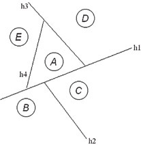
Figure 55.18Objects in a plane.
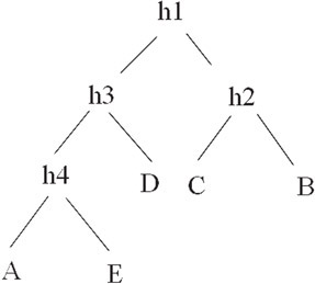
Figure 55.19BSP tree for Figure 55.18.
Note how each vertex can be located relative to at least two planes. For a viewpoint along h3, it is immediately apparent that vertex D is on the right, while A and E are on the left. Vertices C and B are located in the half space of h1 and h2, and are therefore of no interest. Vertices C and B will not be rendered. This relative method works for all positions in the BSP tree.
As mentioned, BSP trees are not a universal solution for hidden surface removal, mainly because of the pre-processing requirement. There is a major caveat; if the objects in the scene are moving, the pre-processing of the BSP tree is no longer valid as the polygons change relative position. The tree must be built every time the relative positions of objects within the tree change. Re-calculating the tree at each time step is often too slow, especially in 3-D gaming, where several million polygons must be rendered every second.
Another problem is that the BSP tree works in hidden surface removal only when “no polygon crosses the plane defined by any other polygon.” In other words, no object can be both behind and in front of another object for the BSP sorting algorithm to work. In gaming, it is common for objects to “collide” so this algorithm becomes even less desirable in these unpredictable conditions.
55.4.2Proximity and Collision: Other Applications of the BSP Tree
Although BSP Tree structures are not as useful for determining the rendering order of moving polygons, they have other applications in graphics and gaming. For instance, trees are commonly used for collision detection, line-of sight, and other algorithms where the number of required calculations is lower. Determining between time-steps the relative positions of several (or several hundred) models, rather than several hundred million polygons, is much more feasible with today’s hardware. Enhanced Tree structures are even used in many of today’s more innovative artificial intelligence algorithms for gaming. These structures are used within the game space to quickly determine how an object sees, touches, and ultimately reacts with other objects.
55.4.3More With Trees: CSG Modeling
Another widely used application of tree-based structures is application of Boolean operations to object construction. Constructive Solid Geometry, or CSG, modeling involves the construction of complex objects using only simple, primitive shapes. These shapes are added and subtracted to each other through “set operations,” or “Boolean operations.” The final objects are referred to as “compound,” “Boolean,” or “CSG” objects [5].
Figure 55.20 of a dumbbell illustrates a typical example of a CSG object.
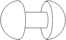
Figure 55.20CSG object.
To construct this object in a CSG environment, Boolean operations are applied to primitive objects. These operations are “intersection,” “union,” and “difference”[5]. Each step in the tree represents a boolean combination between two objects. The resulting object at each point in the tree is then combined again with another Boolean operation at the next step. This type of progression is continued until the finished object is created. Figure 55.21 illustrates the CSG tree used to construct this dumbbell using two spheres, a cylinder, and a half-plane.
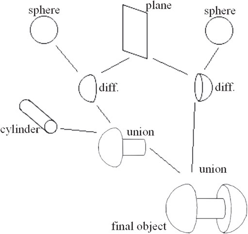
Figure 55.21CSG tree corresponding to Figure 55.20.
A union operation is analogous to gluing two primitives together. An intersection operation results in only the portion (or volume) that both primitives occupy. Finally, a difference operation in effect removes the intersected section of one primitive from another. Armed with these three Boolean operations, modeling and displaying very complex shapes are possible. However, attempting to cover the surface of a final shape with a continuous mesh is another problem entirely, and the subject of numerous texts and papers. Consequently, CSG objects are largely used for initial visualization of a complete model. This solid model is then sent to another application that converts the model to a polygonal mesh.
From a data structure and algorithm standpoint, CSG trees are quite useful. Firstly, and most obvious, the method utilizes the tree structure already mentioned throughout the text. Secondly, the final objects do not require individual mesh models to define them. Rather, each object is simply defined by its tree, where each node of the tree references primitives, such as the sphere, cone, cylinder, cube, and plane. With the basic models for the sphere, cone, etc. preprocessed and stored in memory, the overhead of CSG applications is kept to a minimum.
Many commercially available solid modeling and animation packages still provide CSG as a standard user-interface.
1.Hill, Computer Graphics Using Open GL, 1990, Macmillan Publishing Company.
2.Shirley, Fundamentals of Computer Graphics, 2002, School of Computing University of Utah.
3.Pappas and Murray, Visual Basic Programming with the Windows API, Chapter 15, 1998, Prentice Hall.
4.Arvo, Graphics Gems II, Chapter IV.6, 1991, Academic Press, Inc.
5.Rockwood, Geometric Primitives, 1997, CRC Press Inc.
6.Farin, Curves and Surfaces for CAGD, A Practical Guide, Fifth Edition, 2002, Academic Press.
*This chapter has been reprinted from first edition of this Handbook, without any content updates.
†We have used this author’s affiliation from the first edition of this handbook, but note that this may have changed since then.