
Donghui Zhang†
Northeastern University
16.2The Disk-Based Environment
B-tree Definition•B-tree Query•B-tree Insertion• B-tree Deletion
Copy-up and Push-up•B+-tree Query•B+-tree Insertion•B+-tree Deletion
Efficiency Analysis•Why Is the B+-treeWidely Accepted?•Bulk-Loading a B+-tree•Aggregation Query in a B+-tree
We have seen binary search trees in Chapters 3 and 11. When data volume is large and does not fit in memory, an extension of the binary search tree to disk-based environment is the B-tree, originally invented by Bayer and McCreight [1]. In fact, since the B-tree is always balanced (all leaf nodes appear at the same level), it is an extension of the balanced binary search tree. Since each disk access exchanges a whole block of information between memory and disk rather than a few bytes, a node of the B-tree is expanded to hold more than two child pointers, up to the block capacity. To guarantee worst-case performance, the B-tree requires that every node (except the root) has to be at least half full. An exact match query, insertion or deletion need to access O(logB n) nodes, where B is the page capacity in number of child pointers, and n is the number of objects.
Nowadays, every database management system (see Chapter 62 for more on applications of data structures to database management systems) has implemented the B-tree or its variants. Since the invention of the B-tree, there have been many variations proposed. In particular, Knuth [2] defined the B*-tree as a B-tree in which every node has to be at least 2/3 full (instead of just 1/2 full). If a page overflows during insertion, the B*-tree applies a local redistribution scheme to delay splitting the node till two another sibling node is also full. At this time, the two nodes are split into three. Perhaps the best variation of the B-tree is the B+-tree, whose idea was originally suggested by Knuth [2], but whose name was given by Comer [3]. (Before Comer, Knuth used the name B*-tree to represent both B*-tree and B+-tree.) In a B+-tree, every object stays at the leaf level. Update and query algorithms need to be modified from those of the original B-tree accordingly.
The idea of the B-tree also motivates the design of many other disk-based index structures like the R-tree [4], the state-of-art spatial index structure (Chapter 22).
In this chapter, we describe the B-tree and B+-tree in more detail. In Section 16.2, we briefly describe the disk-based environment and we introduce some notations. The B-tree is described in section 16.3, while the B+-tree is described in Section 16.4. Finally, in Section 16.5 we further discuss some related issues.
16.2The Disk-Based Environment
Most application software deal with data. For instance, a registration application may keep the name, address and social security number of all students. The data has to be stored somewhere. There are three levels of storage. The computer CPU deals directly with the primary storage, which means the main memory (as well as cache). While data stored at this level can be access quickly, we cannot store everything in memory for two reasons. First, memory is expensive. Second, memory is volatile, that is, if there is a power failure, information stored in memory gets lost.
The secondary storage stands for magnetic disks. Although it has slower access, it is less expensive and it is non-volatile. This satisfies most needs. For data which do not need to be accessed often, they can also be stored in the tertiary storage, for example, tapes.
Since the CPU does not deal with disk directly, in order for any piece of data to be accessed, it has to be read from disk to memory first. Data is stored on disk in units called blocks or pages. Every disk access has to read/write one or multiple blocks. That is, even if we need to access a single integer stored in a disk block which contains thousands of integers, we need to read the whole block in. This tells us why internal memory data structures cannot be directly implemented as external-memory index structures.
Consider the binary search tree as an example. Suppose we implement every node as a disk block. The storage would be very inefficient. If a disk page is 8 KB (= 8192 bytes), while a node in the binary search tree is 16 bytes (four integers: a key, a value, and two child pointers), we know every page is only 0.2% full. To improve space efficiency, we should store multiple tree nodes in one disk page. However, the query and update will still be inefficient. The query and update need to access O(log2n) nodes, where n is the number of objects. Since it is possible that every node accessed is stored in a different disk page, we need to access O(log2n) disk pages. On the other hand, the B-tree query/update needs to access only O(logB n) disk pages, which is a big improvement. A typical value of B is 100. Even if there are as many as billions of objects, the height of a B-tree, logB n, will be at most 4 or 5.
A fundamental question that the database research addresses is how to reduce the gap between memory and disk. That is, given a large amount of data, how to organize them on disk in such a way that they can efficiently be updated and retrieved. Here we measure efficiency by counting the total number of disk accesses we make. A disk access can be either a read or a write operation. Without going into details on how the data is organized on disk, let’s make a few assumptions. First, assume each disk page is identified by a number called its pageID. Second, given a pageID, there is a function DiskRead which reads the page into memory. Correspondingly, there is a DiskWrite function which writes the in-memory page onto disk. Third, we are provided two functions which allocate a new disk page and deallocate an existing disk page.
The four functions are listed below.
•DiskRead: given a pageID, read the corresponding disk page into memory and return the corresponding memory location.
•DiskWrite: given the location of an in-memory page, write the page to disk.
•AllocatePage: find an unoccupied pageID, allocate space for the page in memory and return its memory location.
•DeallocatePage: given a pageID, mark the corresponding disk page as being unoccupied.
In the actual implementation, we should utilize a memory buffer pool. When we need to access a page, we should first check if it is already in the buffer pool, and we access the disk only when there is a buffer miss. Similarly, when we want to write a page out, we should write it to the buffer pool. An actual DiskWrite is performed under two circumstances: (a) The buffer pool is full and one page needs to be switched out of buffer. (b) The application program terminates. However, for our purposes we do not differentiate disk access and buffer pool access.
The problem which the B-tree aims to solve is: given a large collection of objects, each having a key and an value, design a disk-based index structure which efficiently supports query and update.
Here the query that is of interest is the exact-match query: given a key k, locate the value of the object with key = k. The update can be either an insertion or a deletion. That is, insert a new object into the index, or delete from the index an object with a given key.
A B-tree is a tree structure where every node corresponds to a disk page and which satisfies the following properties:
•A node (leaf or index) x has a value x.num as the number of objects stored in x. It also stores the list of x.num objects in increasing key order. The key and value of the ith object (1 ≤ i ≤ x.num) are represented as x.key[i] and x.value[i], respectively.
•Every leaf node has the same depth.
•An index node x stores, besides x.num objects, x.num + 1 child pointers. Here each child pointer is a pageID of the corresponding child node. The ith child pointer is denoted as x.child[i]. It corresponds to a key range (x.key[i − 1], x.key[i]). This means that in the ith sub-tree, any object key must be larger than x.key[i − 1] and smaller than x.key[i]. For instance, in the sub-tree referenced by x.child[1], the object keys are smaller than x.key[1]. In the sub-tree referenced by x.child[2], the objects keys are between x.key[1] and x.key[2], and so on.
•Every node except the root node has to be at least half full. That is, suppose an index node can hold up to 2B child pointers (besides, of course, 2B − 1 objects), then any index node except the root must have at least B child pointers. A leaf node can hold more objects, since no child pointer needs to be stored. However, for simplicity we assume a leaf node holds between B and 2B objects.
•If the root node is an index node, it must have at least two children.
A special case of the B-tree is when B = 2. Here every index node must have 2 or 3 or 4 child pointers. This special case is called the 2-3-4 tree.
Figure 16.1 shows an example of a B-tree. In particular, it’s a 2-3-4 tree.

Figure 16.1An example of a B-tree.
In the figure, every index node contains between 2 and 4 child pointers, and every leaf node contains between 2 and 4 objects. The root node A is an index node. Currently it has one object with key = 25 and two child pointers. In the left sub-tree, every object has key < 25. In the right sub-tree, every object has key > 25. Every leaf node (D through I) are located at the same depth: their distance to A is 2. Currently, there are two pages which are full: an index node B and a leaf node D.
To find the value of an object with key = k, we call the Query algorithm given below. The parameters are the tree root pageID and the search key k. The algorithm works as follows. It follows (at most) a single path from root to leaf. At each index node along the path, there can be at most one sub-tree whose key range contains k. A recursive call on that sub-tree is performed (step 2c). Eventually, we reach a leaf node (step 3a). If there exists an object in the node with key = k, the algorithm returns the value of the object. Otherwise, the object does not exist in the tree and NULL is returned. Since the index nodes of the B-tree also stores objects, it is possible that the object with key = k is found in an index node. In this case, the algorithm returns the object value without going down to the next level (step 2a).
Algorithm Query(pageID, k)
Input: pageID of a B-tree node, a key k to be searched.
Output: value of the object with key = k; NULL if non-exist.
1.x = DiskRead(pageID).
2.if x is an index node
a.If there is an object o in x s.t. o.key = k, return o.value.
b.Find the child pointer x.child[i] whose key range contains k.
c.return Query(x.child[i], k).
3.else
a.If there is an object o in x s.t. o.key = k, return o.value. Otherwise, return NULL.
4.end if
As an example, Figure 16.2 shows how to perform a search query for k = 13. At node A, we should follow the left sub-tree since k < 25. At node B, we should follow the third sub-tree since 10 < k < 16. Now we reach a leaf node F. An object with key = 13 is found in the node.

Figure 16.2Query processing in a B-tree.
If the query wants to search for k = 12, we still examine the three nodes A, B, F. This time, no object with key = 12 is found in F, and thus the algorithm returns NULL. If the search key is 10 instead, the algorithm only examines node A and B. Since in node B such an object is found, the algorithm stops there.
Notice that in the Query algorithm, only DiskRead function is called. The other three functions, for example, DiskWrite are not needed as the algorithm does not modify the B-tree. Since the query algorithm examines a single path from root to leaf, the complexity of the algorithm in number of I/Os is O(logB n), where n is the number of objects.
To insert a new object with key k and value v into the index, we call the Insert algorithm given below.
Algorithm Insert(root, k, v)
Input: root pageID of a B-tree, the key k and the value v of a new object.
Prerequisite: The object does not exist in the tree.
Action: Insert the new object into the B-tree.
1.x = DiskRead(root).
2.if x is full
a.y = AllocatePage(), z = AllocatePage().
b.Locate the middle object oi stored in x. Move the objects to the left of oi into y. Move the objects to the right of oi into z. If x is an index page, also move the child pointers accordingly.
c.x.child[1] = y.pageID, x.child[2] = z.pageID.
d.DiskWrite(x), DiskWrite(y), DiskWrite(z).
3.end if
4.InsertNotFull(x, k, v).
Basically, the algorithm makes sure that root page is not currently full, and then it calls the InsertNotFull function to insert the object into the tree. If the root page x is full, the algorithm will split it into two nodes y and z, and node x will be promoted to a higher level, thus increasing the height of the tree.
This scenario is illustrated in Figure 16.3. Node x is a full root page. It contains three objects and four child pointers. If we try to insert some record into the tree, the root node is split into two nodes y and z. Originally, x contains x.num = 3 objects. The left object (key = 6) is moved to a new node y. The right object (key = 16) is moved to a new node z. The middle object (key = 10) remains in x. Correspondingly, the child pointers D, E, F, G are also moved. Now, x contains only one object (key = 10). We make it as the new root, and make y and z be the two children of it.

Figure 16.3Splitting the root node increases the height of the tree.
To insert an object into a sub-tree rooted by a non-full node x, the following algorithm InsertNotFull is used.
Algorithm InsertNotFull(x, k, v)
Input: an in-memory page x of a B-tree, the key k and the value v of a new object.
Prerequisite: page x is not full.
Action: Insert the new object into the sub-tree rooted by x.
1.if x is a leaf page
a.Insert the new object into x, keeping objects in sorted order.
b.DiskWrite(x).
2.else
a.Find the child pointer x.child[i] whose key range contains k.
b.w = DiskRead(x.child[i]).
c.if w is full
i.y = AllocatePage().
ii.Locate the middle object oj stored in w. Move the objects to the right of oj into y. If w is an index page, also move the child pointers accordingly.
iii.Move oj into x. Accordingly, add a child pointer in x (to the right of oj) pointing to y.
iv.DiskWrite(x), DiskWrite(y), DiskWrite(w).
v.If k < oj.key, call InsertNotFull(w, k, v); otherwise, call InsertNotFull(y, k, v).
d.else
InsertNotFull(w, k, v).
e.end if
3.end if
Algorithm InsertNotFull examines a single path from root to leaf, and eventually insert the object into some leaf page. At each level, the algorithm follows the child pointer whose key range contains the key of the new object (step 2a). If no node along the path is full, the algorithm recursively calls itself on each of these nodes (step 2d) till the leaf level, where the object is inserted into the leaf node (step 1).
Consider the other case when some node w along the path is full (step 2c). The node is first split into two (w and y). The right half of the objects from w are moved to y, while the middle object is pushed into the parent node. After the split, the key range of either w or y, but not both, contains the key of the new object. A recursive call is performed on the correct node.
As an example, consider inserting an object with key = 14 into the B-tree of Figure 16.2. The result is shown in Figure 16.4. The child pointers that are followed are thick. When we examine the root node A, we follow the child pointer to B. Since B is full, we first split it into two, by moving the right half of the objects (only one object in our case, with key = 16) into a new node B′′. The child pointers to F and G are moved as well. Further, the previous middle object in B (key = 10) is moved to the parent node A. A new child pointer to B′′ is also generated in A. Now, since the key of the new object is 14, which is bigger than 10, we recursively call the algorithm on B′′. At this node, since 14 < 16, we recursively call the algorithm on node F. Since F is a leaf node, the algorithm finishes by inserting the new object into F. The accessed disk pages are shown as shadowed.
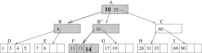
Figure 16.4Inserting an object with key = 14 into the B-tree of Figure 16.2 Since node B is full, it is split into two (B and B′′). The object is recursively inserted into the sub-tree rooted by B′′. At the lowest level, it is stored in node F.
This section describes the Delete algorithm which is used to delete an object with key = k from the B-tree. It is a recursive algorithm. It takes (besides k) as parameter a tree node, and it will perform deletion in the sub-tree rooted by that node.
We know that there is a single path from the root node to the node x that contains k. The Delete algorithm examines this path. Along the path, at each level when we examine node x, we first make sure that x has at least one more element than half full (except the case when x is the root). The reasoning behind this is that in order to delete an element from the sub-tree rooted by x, the number of element stored in x can be reduced at most by one. If x has one more element than half full (minimum occupancy), it can be guaranteed that x will not underflow. We distinguish three cases:
1.x is a leaf node;
2.x is an index node which contains an object with key = k;
3.x is an index node which does not contain an object with key = k.
We first describe the Delete algorithm and then discuss the three cases in more detail.
Algorithm Delete(x, k)
Input: an in-memory node x of a B-tree, the key k to be deleted.
Prerequisite: an object with key = k exists in the sub-tree rooted by x.
Action: Delete the object from the sub-tree rooted by x.
1.if x is a leaf page
a.Delete the object with key = k from x.
b.DiskWrite(x).
2.else if x does not contain the object with key = k
a.Locate the child x.child[i] whose key range contains k.
b.y = DiskRead(x.child[i]).
c.if y is exactly half full
i.If the sibling node z immediate to the left (right) of y has at least one more object than minimally required, add one more object to y by moving x.key[i] from x to y and move that last (first) object from z to x. If y is an index node, the last (first) child pointer in z is also moved to y.
ii.Otherwise, any immediate sibling of y is exactly half full. Merge y with an immediate sibling.
end if
d.Delete(y, k).
3.else
a.If the child y that precedes k in x has at least one more object than minimally required, find the predecessor k′ of k in the sub-tree rooted by y, recursively delete k′ from the sub-tree and replace k with k′ in x.
b.Otherwise, y is exactly half full. We check the child z that immediately follows k in x. If z has at least one more object than minimally required, find the successor k′ of k in the sub-tree rooted by z, recursively delete k′ from the sub-tree and replace k with k′ in x.
c.Otherwise, both y and z are half full. Merge them into one node and push k down to the new node as well. Recursively delete k from this new node.
4.end if
Along the search path from the root to the node containing the object to be deleted, for each node x we encounter, there are three cases. The simplest scenario is when x is a leaf node (step 1 of the algorithm). In this case, the object is deleted from the node and the algorithm returns. Note that there is no need to handle underflow. The reason is: if the leaf node is root, there is only one node in the tree and it is fine if it has only a few objects; otherwise, the previous recursive step has already guaranteed that x has at least one more object than minimally required.
Steps 2 and 3 of the algorithm correspond to two different cases of dealing with an index node.
For step 2, the index node x does not contain the object with key = k. Thus there exists a child node y whose key range contains k. After we read the child node into memory (step 2b), we will recursively call the Delete algorithm on the sub-tree rooted by y (step 2d). However, before we do that, step 2(c) of the algorithm makes sure that y contains at least one more object than half full.
Suppose we want to delete 5 from the B-tree shown in Figure 16.2. When we are examining the root node A, we see that child node B should be followed next. Since B has two more objects than half full, the recursion goes to node B. In turn, since D has two more objects than minimum occupancy, the recursion goes to node D, where the object can be removed.
Let’s examine another example. Still from the B+-tree shown in Figure 16.2, suppose we want to delete 33. The algorithm finds that the child node y = C is half full. One more object needs to be incorporated into node C before a recursive call on C is performed. There are two sub-cases. The first sub-case is when one immediate sibling z of node y has at least one more object than minimally required. This case corresponds to step 2(c)i of the algorithm. To handle this case, we drag one object down from x to y, and we push one object from the sibling node up to x. As an example, the deletion of object 33 is shown in Figure 16.5.
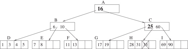
Figure 16.5Illustration of step 2(c)i of the Delete algorithm. Deleting an object with key = 33 from the B-tree of Figure 16.2. At node A, we examine the right child. Since node C only had one object before, a new object was added to it in the following way: the object with key = 25 is moved from A to C, and the object with key = 16 is moved from B to A. Also, the child pointer pointing to G is moved from B to C.
Another sub-case is when all immediate siblings of y are exactly half full. In this case, we merge y with one sibling. In our 2-3-4-tree example, an index node which is half full contains one object. If we merge two such nodes together, we also drag an object from the parent node of them down to the merged node. The node will then contain three objects, which is full but does not overflow.
For instance, suppose we want to delete object 31 from Figure 16.5. When we are examining node x = C, we see that we need to recursively delete in the child node y = H. Now, both immediate siblings of H are exactly half full. So we need to merge H with a sibling, say G. Besides moving the remaining object 28 from H to G, we also should drag object 25 from the parent node C to G. The figure is omitted for this case.
The third case is that node x is an index node which contains the object to be deleted. Step 3 of algorithm Delete corresponds to this scenario. We cannot simply delete the object from x, because we also need to decrement the number of child pointers by one. In Figure 16.5, suppose we want to delete object with key = 25, which is stored in index node C. We cannot simply remove the object, since C would have one object but three child pointers left. Now, if child node G immediately to the left of key 25 had three or more objects, the algorithm would execute step 3(a) and move the last object from G into C to fill in the space of the deleted object. Step 3(b) is a symmetric step which shows that we can move an object from the right sub-tree.
However, in our case, both child nodes G and H are half full and thus cannot contribute an object. Step 3(c) of the algorithm corresponds to this case. As shown in Figure 16.6, the two nodes are merged into one.

Figure 16.6Illustration of step 3(c) of the Delete algorithm. Deleting an object with key = 25 from the B-tree of Figure 16.5. At node A, we examine the right child. We see that node C contains the object with key = 25. We cannot move an object up from a child node of C, since both children G and H (around key 25) are exactly half full. The algorithm merges these two nodes into one, by moving objects 28 and 31 from H to G and then deleting H. Node C loses an object (key = 25) and a child pointer (to H).
The most well-know variation of the B-tree is the B+-tree. There are two major differences from the B-tree. First, all objects in the B+-tree are kept in leaf nodes. Second, all leaf nodes are linked together as a double-linked list.
The structure of the B+-tree looks quite similar to the B-tree. Thus we omit the details. We do point out that in an index node of a B+-tree, different from the B-tree, we do not store object values. We still store object keys, though. However, since all objects are stored in the leaf level, the keys stored in index nodes act as routers, as they direct the search algorithm to go to the correct child node at each level.
One may wonder where the routers in the index nodes come from. To understand this, let’s look at an example. Initially, the B+-tree has a single node which is a leaf node. After 2B insertions, the root node becomes full. In Figure 16.7a, if we try to insert an object to the node A when it is already full, it temporarily overflows. To handle the overflow, the B+-tree will split the node into two nodes A and B. Furthermore, a new node C is generated, which is the new root of the tree. The first key in leaf node B is copied up to C. The result B+-tree is shown in Figure 16.7b.

Figure 16.7Illustration of a leaf-node split in the B+-tree. The middle key 40 (same as the first key in the right node) is copied up to the parent node.
We point out that a key in an index node may be validly replaced by some other keys, unlike in a leaf node. For instance, in node C of Figure 16.7b, we can replace the key 40–35. As long as it is smaller than all keys in the left sub-tree and bigger than or equal to all keys in the right sub-tree, it is fine.
To emphasize the fact that the keys in a index node are different from the keys in a leaf node (a key in an index node is not a real object), in the B+-tree figures we will attach a (*) to each key in a leaf node.
As a comparison, consider the split of an index node. In Figure 16.8a, the index node C temporarily overflows. It is split into two, C and G. Since before the split, C was the tree root, a new root node H is generated. See Figure 16.8b. Here the middle key 51 in the original node C is pushed up to the parent node.

Figure 16.8Illustration of an index-node split in the B+-tree. The middle key 51 is pushed up to the parent node.
As in the B-tree, the B+-tree supports the exact-match query which finds the object with a given key. Furthermore, the B+-tree can efficiently support the range query, which finds the objects whose keys are in a given range.
To perform the exact-match query, the B+-tree follows a single path from root to leaf. In the root node, there is a single child pointer whose key range contains the key to be searched for. If we follow the child pointer to the corresponding child node, inside the child node there is also a single child pointer whose key range contains the object to be searched for. Eventually, we reach a leaf node. The object to be searched, if it exists, must be located in this node. As an example, Figure 16.9 shows the search path if we search key = 42.

Figure 16.9Illustration of the exact-match query algorithm in the B+-tree. To search for an object with key = 42, nodes H, C and B are examined.
Beside the exact-match query, the B+-tree also supports the range query. That is, find all objects whose keys belong to a range R. In order to do so, all the leaf nodes of a B+-tree are linked together. If we want to search for all objects whose keys are in the range R = [low, high], we perform an exact match query for key = low. This leads us to a leaf node l. We examine all objects in l, and then we follow the sibling link to the next leaf node, and so on. The algorithm stops when an object with key > high is met. An example is shown in Figure 16.10.

Figure 16.10Illustration of the range query algorithm in the B+-tree. To search for all objects with keys in the range [42,75], the first step is to follow a path from root to leaf to find key 42 (H, C and B are examined). The second step is to follow the right-sibling pointers between leaf nodes and examine D, E. The algorithm stops at E as an object with key = 76 is found.
Since all objects in the B+-tree are located at the leaf level, the insertion algorithm of the B+-tree is actually easier than that in the B-tree. We basically follow the exact-match query to find the leaf node which should contain the object if it were in the tree. Then we insert the object into the leaf node.
What needs to be taken care of is when the leaf node overflows and is split into two. In this case, a key and a child pointer are inserted into the parent node. This may in turn cause the parent node to overflow, and so on. In the worst case, all nodes along the insertion path are split. If the root node splits into two, the height of the tree increases by one. The insertion algorithm is given below.
Algorithm Insert(root, k, v)
Input: the root pageID of a B+-tree, the key k and the value v of a new object.
Prerequisite: the object with key = k does not exist in the tree.
Action: Insert the new object into the B+-tree.
1.Starting with the root node, perform an exact-match for key = k till a leaf node. Let the search path be x1, x2, …, xh, where x1 is the root node, xh is the leaf node where the new object should be inserted into, and xi is the parent node of xi + 1 where 1 ≤ i ≤ h-1.
2.Insert the new object with key = k and value = v into xh.
3.Let i = h.
4.while xi overflows
a.Split xi into two nodes, by moving the larger half of the keys into a new node xi′. If xi is a leaf node, link xi′ into the double-linked list among leaf nodes.
b.Identify a key kk to be inserted into the parent level along with the child pointer pointing to xi′. The choice of kk depends on the type of node xi. If xi is a leaf node, we need to perform Copy-up. That is, the smallest key in xi′ is copied as kk to the parent level. On the other hand, if xi is an index node, we need to perform Push-up. This means the smallest key in xi′ is removed from xi′ and then stored as kk in the parent node.
c.if i = = 1 /* the root node overflows */
i.Create a new index node as the new root. In the new root, store one key = kk and two child pointers to xi and xi′.
ii.return
d.else
i.Insert a key kk and a child pointer pointing to xi′ into node xi−1.
ii.i = i − 1.
e.end if
5.end while
As an example, Figure 16.11 shows how to insert an object with key = 60 into the B+-tree shown in Figure 16.9.

Figure 16.11After inserting an object with key = 60 into the B+-tree shown in Figure 16.9. Leaf node D splits into two. The middle key 56 is copied up to the parent node G.
To delete an object from the B+-tree, we first examine a single path from root to the leaf node containing the object. Then we remove the object from the node. At this point, if the node is at least half full, the algorithm returns. Otherwise, the algorithm tries to re-distribute objects between a sibling node and the underflowing node. If redistribution is not possible, the underflowing node is merged with a sibling.
Algorithm Delete(root, k)
Input: the root pageID of a B+-tree, the key k of the object to be deleted.
Prerequisite: the object with key = k exists in the tree.
Action: Delete the object with key = k from the B+-tree.
1.Starting with the root node, perform an exact-match for key = k. Let the search path be x1, x2, …, xh, where x1 is the root node, xh is the leaf node that contains the object with key = k, and xi is the parent node of xi + 1. (1 ≤ i ≤ h − 1)
2.Delete the object with key = k from xh.
3.If h = = 1, return. This is because the tree has only one node which is the root node, and we do not care whether a root node underflows or not.
4.Let i = h.
while xi underflows
a.if an immediate sibling node s of xi has at least one more entry than minimum occupancy
i.Re-distribute entries evenly between s and xi.
ii.Corresponding to the re-distribution, a key kk in the parent node xi − 1 needs to be modified. If xi is an index node, kk is dragged down to xi and a key from s is pushed up to fill in the place of kk. Otherwise, kk is simply replaced by a key in s.
iii.return
b.else
i.Merge xi with a sibling node s. Delete the corresponding child pointer in xi − 1.
ii.If xi is an index node, drag the key in xi − 1, which previously divides xi and s, into the new node xi. Otherwise, delete that key in xi − 1.
iii.i = i − 1.
c.end if
end while
Step 1 of the algorithm follows a single path from root to leaf to find the object to be deleted. Step 2 deletes the object. The algorithm will finish at this point if any of the following two conditions hold. One, if the tree has a single node (step 3). Two, the leaf node is at least half full after the deletion (the while loop of step 4 is skipped).
As an example, suppose we delete object 56 and then 62 from the B+-tree shown in Figure 16.9. The deletions go to the same leaf node D, where no underflow occurs. The result is shown in Figure 16.12.

Figure 16.12After deleting keys 56 and 62 from the B+-tree of Figure 16.9. Both keys are deleted from leaf node D, which still satisfies the minimum occupancy.
Now, let’s try to delete key 53 from Figure 16.12. This time D underflows. Step 4 of the Delete algorithm handles underflows. In general, when a node xi underflows, the algorithm tries to borrow some entries from a sibling node s, as described in step 4(a). Note that we could borrow just one entry to avoid underflow in xi. However, this is not good because next time we delete something from xi, it will underflow again. Instead, the algorithm redistribute entries evenly between xi and s. Assume xi has B − 1 objects and s has B + k objects, where k ∈ [1..B]. After redistribution, both xi and s will have B + (k − 1)/2 objects. Thus xi can take another (k − 1)/2 deletions before another underflow occurs.
In our example, to delete key 53 from node D, we re-distribute objects in D and E, by moving 72* into D. As discussed in step 4(a)ii of the algorithm, we also needs to modify a key in the parent node G. In our case, since D is a leaf node, we simply replace the key 72 by 75 in node G. Here 75 is the smallest key in E. The result after the redistribution is shown in Figure 16.13. As a comparison, consider the hypothetical case when D were an index node. In this case, we would drag down the key 72 from G to D and push up a key from E to G.

Figure 16.13After deleting keys 53 from Figure 16.12. Objects in D and E are redistributed. A key in G is modified.
Let’s proceed the example further by deleting object 72 from the tree in Figure 16.13. Now, the node D underflows, and redistribution is not possible (since E, the only immediate sibling of D, is exactly half full). Step 4(b) of the Delete algorithm tells us to merge D and E together. Correspondingly, a key and a child pointer need to be deleted from the parent node G. Since D is a leaf node, we simply delete the key 75 and the child pointer from G. The result is shown in Figure 16.14. As a comparison, imagine D were an index node. We would still remove key 75 and the child pointer from G, but we would keep the key 75 in node D.

Figure 16.14After deleting keys 72 from Figure 16.13. This figure corresponds to the scenario described in step 4(b) of the Delete algorithm. In particular, the example illustrates the merge of two leaf nodes (D and E). Node D underflows, but redistribution is not possible. From the parent node G, key 75 and child pointer to E are removed.
One may wonder why in the redistribution and the merge algorithms, the leaf node and the index node are treated differently. The reason is because when we generated an index entry, we had treated two cases differently: the case when the entry points to a leaf node and the case when the entry points to a index node. This is discussed at the beginning of Section 16.4. To generate a new entry pointing to a leaf node, we copied the smallest key from the leaf node. But to generate a new entry pointing to an index node, we pushed a key from the child node up. A key which was copied up can be safely deleted later (when merge occurs). But a key which was pushed up must be kept somewhere. If we delete it from a parent node, we should drag it down to a child node.
As a running example of merging index nodes, consider deleting object 42 from the B+-tree of Figure 16.14. Node B underflows, and it is merged with A. Correspondingly, in the parent node C, the key 40 and the child pointer to B are deleted. The temporary result is shown in Figure 16.15. It’s temporary since node C underflows.

Figure 16.15Temporary tree in the middle of deleting object 42 from Figure 16.14. Nodes A and B are merged. Key 40 and child pointer to B are removed from C.
To handle the underflow of node C, it is merged with G, its sole sibling node. As a consequence, the root node H now has only one child. Thus, H is removed and C becomes the new root. We point out that to merge two index nodes C and G, a key is dragged down from the parent node (versus being deleted in the case of merging leaf nodes). The final result after completing the deletion of 42* is shown in Figure 16.16.

Figure 16.16After the deletion of object 42 is finished. This figure illustrates an example of merging two index nodes. In particular, index nodes C and G are merged. The key 51 is dragged down from the parent node H. Since that is the only key in root H, node C becomes the new root and the height of the tree is decreased by one.
In this section we discuss various issues of the B-tree and the B+-tree.
Theorem: In the B-tree or the B+-tree, the I/O cost of insertion, deletion and exact-match query is O(logB n). In the B+-tree, the I/O cost of a range search is O(logB n + t/B). Here B is the minimum page capacity in number of records, n is the total number of objects in the tree, and t is the number of objects in the range query result.
The correctness of the theorem can be seen from the discussion of the algorithms. Basically, for both the B-tree and the B+-tree, all the insertion, deletion and exact-match query algorithms examine a single path from root to leaf. At each node, the algorithm might examine up to two other nodes. However, asymptotically the complexity of these algorithms are equal to the height of the tree. Since there are n objects, and the minimum fan-out of the tree is B, the height of the tree is O(logBn). So the complexity of the algorithms is O(logBn) as well.
For the range query in the B+-tree, logBn nodes are examined to find the leaf node that contains the low value of the query range. By following the sibling pointers in the leaf nodes, the other leaf nodes that contain objects in the query range are also found. Among all the leaf nodes examined, except for the first and the last, every node contains at least B objects in the query result. Thus if there are t objects in the query result, the range query complexity is O(logBn + t/B).
16.5.2Why Is the B+-tree Widely Accepted?
One can safely claim that the B+-tree has been included in at least 99%, if not all, of the database management systems (DBMS). No other index structure has received so much attention. Why is that?
Let’s do some calculation. First, we point out that a practical number of minimum occupancy of a B+-tree is B = 100. Thus the fan-out of the tree is between 100 and 200. Analysis has shown that in a real-world B+-tree, the average page capacity is about 66.7% full. Or, a page typically contains 200*66.7% = 133 entries. Here is the relationship between the height of the tree and the number of objects that can hold in a typical B+-tree:
•height = 0: B+-tree holds 133 objects on average. There is a single node, which is 66.7% full.
•height = 1: B+-tree holds 1332 = 17, 689 objects. There are 133 leaf nodes, each holds 133 objects.
•height = 2: B+-tree holds 1333 = 2, 352, 637 objects.
•height = 3: B+-tree holds 1334 = 312, 900, 721 (over 0.3 billion) objects.
The first two levels of the B+-tree contains 1 + 133 = 134 disk pages. This is very small. If a disk page is 4 KB large, 134 disk pages occupy 134*4 KB = 536 KB disk space. It’s quite reasonable to assume that the first two levels of the B+-tree always stays in memory.
The calculations lead to this discovery: in a large database with 0.3 billion objects, to find one object we only need to access two disk pages! This is unbelievably good.
In some cases, we are given a large set of records and we are asked to build a B+-tree index. Of course, we can start with an empty B+-tree and insert one record at a time using the Insert algorithm. However, this approach is not efficient, as the I/O cost is O(n· logB n).
Many systems have implemented the bulk-loading utility. The idea is as follows. First, sort the objects. Use the objects to fill in leaf nodes in sequential order. For instance, if a leaf node holds up to 2B objects, the 2B smallest objects are stored in page 1, the next 2B objects are stored in page 2, etc. Next, build the index nodes at one level up. Assume an index node holds up to 2B child pointers. Create the first index node as the parent of the first 2B leaf nodes. Create the second index node as the parent of the next 2B leaf nodes, etc. Then, build the index nodes at two levels above the leaf level, and so on. The process stops when there is only one node at a level. This node is the tree root.
If the objects are sorted already, the bulk-loading algorithm has an I/O cost of O(n/B). Otherwise, the bulk-loading algorithm has asymptotically the same I/O cost as external sort, which is O(n/B· logB n). Notice that even if the bulk-loading algorithm performs a sorting first, it is still B times faster than inserting objects one at a time into the structure.
16.5.4Aggregation Query in a B+-tree
The B+-tree can also be used to answer the aggregation query: “given a key range R, find the aggregate value of objects whose keys are in R.” The standard SQL supports the following aggregation operators: COUNT, SUM, AVG, MIN, MAX. For instance, the COUNT operator returns the number of objects in the query range. Here AVG can be computed as SUM/AVG. Thus we focus on the other four aggregate operators.
Since the B+-tree efficiently supports the range query, it makes sense to utilize it to answer the aggregation query as well. Let’s first look at some concepts.
Associated with each aggregate operator, there exists a init_value and an aggregate function. The init_value is the aggregate for an empty set of objects. For instance, the init_value for the COUNT operator is 0. The aggregate function computes the aggregate value. There are two versions. One version takes two aggregate values of object set S1 and S2, and computes the aggregate value of set S1∪ S2. Another version takes one aggregate value of set S1 and an object o and computes the aggregate value of S1∪ {o}. For instance, if we know COUNT1 and COUNT2 of two sets, the COUNT for the whole set is COUNT1 + COUNT2. The COUNT of subset 1 added with an object o is COUNT1 + 1. The init_value and the aggregate functions for COUNT, SUM, MIN, and MAX are shown below.
•COUNT operator:
•init_value = 0
•aggregate(COUNT1, COUNT2) = COUNT1 + COUNT2
•aggregate(COUNT1, object) = COUNT1 + 1
•SUM operator:
•init_value = 0
•aggregate(SUM1, SUM2) = SUM1 + SUM2
•aggregate(SUM1, object) = SUM1 + object.value
•MIN operator:
•init_value = + ∞
•aggregate(MIN1, MIN2) = min{MIN1, MIN2}
•aggregate(MIN1, object) = min{MIN1, object.value}
•MAX operator:
•init_value = − ∞
•aggregate(MAX1, MAX2) = max{MAX1, MAX2}
•aggregate(MAX1, object) = max{MAX1, object.value}
The B+-tree can support the aggregation query in the following way. We keep a temporary aggregate value, which is initially set to be init_value. A range search is performed on the B+-tree. For each object found, its value is aggregated with the temporary aggregate value on-the-fly. When all objects whose keys are in the query range are processed, this temporary aggregate value is returned.
However, this approach is not efficient, as the I/O cost is O(logB n + t/B), which is linear to the number of objects divided by B. If the query range is large, the algorithm needs to access too many disk pages. It is ideal to find some approach whose query performance is independent to the size of the objects in the query range.
A better way is to store the local aggregate values in the tree. In more detail, along with each child pointer, we store the aggregate value of all objects in the corresponding sub-tree. By doing so, if the query range fully contains the key range of a sub-tree, we take the associated local aggregate value and avoid browsing the sub-tree. We call such a B+-tree with extra aggregate information the aggregation B+-tree. The algorithm to perform a aggregation query using the aggregation B+-tree is shown below.
Algorithm Aggregation(x, R)
Input: a node x of an aggregation B+-tree, the query key range R.
Action: Among objects in the sub-tree rooted by x, compute the aggregate value of objects whose keys belong to R.
1.Initialize the temporary aggregation value v as init_value.
2.if x is a leaf node
a.For every object o in x where o.value ∈ R, v = aggr(v, o).
3.else
a.for every child pointer x.child[i]
i.if the key range of x.child[i] is contained in R
v = aggregate(v, x.child[i].aggr)
ii.else if the key range of x.child[i] intersects R
y = DiskRead(x.child[i])
v = aggregate(v, Aggregation(y, R))
iii.end if
b.end for
4.return v.
The algorithm starts with examining the root node. Here the child pointers are divided into three groups. (1) There are at most two child pointers whose key ranges intersect the query range R. (2) The child pointers between them have key ranges fully contained in R. (3) The child pointers outside of them have key ranges non-intersecting with R.
For child pointers in group (2), the local aggregate stored at the child pointer (represented by x.child[i].aggr) is aggregated to the temporary aggregate value and the examination of the sub-tree is avoided. This is shown in step 3(a)i of the algorithm. For child pointers in group (3), no object in the sub-trees will contribute to the query and the examination of the sub-trees are also avoided.
For each of the two child pointers whose key ranges intersect R, a recursive call to Aggregation is performed. This is shown in step 3(a)ii of the algorithm. If we go one level down, in each of the two child nodes, there can be at most one child pointer whose key range intersects R. Take the left child node as an example. If there is a child pointer whose key range intersect R, all child pointers to the left of it will be outside of R and all child pointers to the right of it will be fully contained in R. Thus the algorithm examines two paths from root to leaf.
Theorem: The I/O cost of the Aggregation query algorithm is O(logB n).
The above theorem shows that the aggregation query performance is independent of the number of objects in the query range.
1.R. Bayer and E. M. McCreight: Organization and maintenance of large ordered indices. Acta Informatica, 1, 1972.
2.D. Knuth: The Art of Computer Programming, Vol. 3: Sorting and Searching. Reading, MA: Addison Wesley, 1973.
3.D. Comer: The Ubiquitous B-Tree. ACM Computing Surveys, 11(2), 1979.
4.A. Guttman: R-trees: A dynamic index structure for spatial searching. In Proceedings of ACM/SIGMOD Annual Conference on Management of Data (SIGMOD), 1984.
*This chapter has been reprinted from first edition of this Handbook, without any content updates.
†We have used this author’s affiliation from the first edition of this handbook, but note that this may have changed since then.