22. R-Trees

Spatial database management systems must be able to store and process large amounts of disk-resident spatial data. Multidimensional data support is needed in many fields including geographic information systems (GIS), computer aided design (CAD), and medical, multimedia, and scientific databases. Spatial data operations that need to be supported include spatial joins and various types of queries such as intersection, containment, topological and proximity queries. The challenge, and primary performance objective, for applications dealing with disk-resident data is to minimize the number of disk retrievals, or I/Os, needed to answer a query. Main memory data structures are designed to reduce computation time rather than I/O, and hence are not directly applicable to a disk based environment.

Just as the B-tree [1] (Chapter 16) and its variants were proposed to optimize I/O while processing single dimensional disk resident data, the original R-tree [2] and later variants have been proposed to index disk resident multidimensional data efficiently.

R-trees are very versatile, in the sense that they can be used with little or no modification to tackle many different problems related to spatial data. Asymptotically better data structures exist for specific instances of these problems, but the solution of choice is different for different types of inputs or queries. Thus, one of the main advantages of R-trees is that the same data structure can be used to handle different problems on arbitrary types of multidimensional data.

In this chapter we describe the original R-tree proposal and some of its variants. We analyze the efficiency of various operations and examine various performance models. We also describe R-tree based algorithms for additional operations, such as proximity queries and spatial joins. There are many more applications, variants and issues related to R-trees than we can possibly cover in one chapter. Some of the ones we do not cover include parallel and distributed R-trees [3–6], variants for high dimensional [7–9] and for spatio-temporal data [10–16], and concurrency [17,18]. See Chapter 48 for more on concurrent data structures. Other data structures with similar functionality, such as range, quad and k-d trees, are covered in other chapters of Part IV of this handbook. Some of these (see Chapter 28) are specifically designed for disk-resident data.

22.2Basic Concepts

R-trees were first introduced in Reference 2. An R-tree is a hierarchical data structure derived from the B⁺-tree and originally designed to perform intersection queries efficiently. The tree stores a collection of d-dimensional points or rectangles which can change in time via insertions and deletions. Other object types, such as polygons or polyhedra, can be handled by storing their minimum bounding rectangles (MBRs) and performing additional tests to eliminate false hits. A false hit happens when the query object intersects the MBR of a data object but does not intersect the object itself. In the sequel we talk about rectangles only, with the understanding that a point is simply a degenerate rectangle. We use the terms MBR and bounding box, interchangeably. In our context, the d-dimensional rectangles are “upright,” that is, each rectangle is the Cartesian product of d one-dimensional intervals: [l1, h1] × ··· × [l_d, h_d]. Thus, 2d values are used to specify a rectangle.

Each node of the tree stores a maximum of B entries. With the exception of the root, each node also stores a minimum of b ≤ B/2 entries. This constraint guarantees a space utilization of at least b/B. Each entry E consists of a rectangle r and a pointer p_r. As with B⁺-trees all input values are stored at the leaves. Thus, at the leaf level, r is the bounding box of an actual object pointed to by p_r. At internal nodes, r is the bounding box of all rectangles stored in the subtree pointed to by p_r.

A downward path in the tree corresponds to a sequence of nested rectangles. All leaf nodes occur at the same level (i.e., have the same depth), even after arbitrary sequences of updates. This guarantees that the height of the tree is O(log_bn), where n is the number of input rectangles. Notice that MBRs at the same level may overlap, even if the input rectangles are disjoint.

Figure 22.1 illustrates an R-tree with 3 levels (the root is at level 0) and a maximum of B = 4 rectangles per node. The 64 small dark data rectangles are grouped into 16 leaf level nodes, numbered 1 –16. The bounding box of the set of rectangles stored at the same node is one of the rectangles stored at the parent of the node. In our example, the MBRs of leaf level nodes 1 through 4 are placed in node 17, in level 1. The root node contains the MBRs of the four level 1 nodes: 17, 18, 19, and 20.

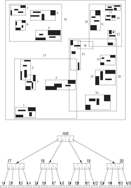
Figure 22.1A sample R-tree using B = 4. Input rectangles are shown solid.

22.2.1Intersection Queries

To perform an intersection query Q, all rectangles that intersect the query region must be retrieved and examined (regardless of whether they are stored in an internal node or a leaf node). This retrieval is accomplished by using a simple recursive procedure that starts at the root node and which may follow multiple paths down the tree. In the worst case, all nodes may need to be retrieved, even though some of the input data need not be reported. A node is processed by first identifying all the rectangles stored at that node which intersect Q. If the node is an internal node, the subtrees corresponding to the identified rectangles are searched recursively. Otherwise, the node is a leaf node and the retrieved rectangles (or the data objects themselves) are simply reported.

For illustration, consider the query Q in the example of Figure 22.1. After examining the root node, we determine that nodes 19 and 20 of level 1 must be searched. The search then proceeds with each of these nodes. Since the query region does not intersect any of the MBRs stored in node 19, this sub-query is terminated. While processing the other sub-query, it is determined that Q intersects the MBR corresponding to node 13 and this node is retrieved. Upon checking the rectangles in node 13, the one data rectangle intersected by Q is returned.

Other type of queries, such as arbitrarily shaped queries (e.g., point or polygonal queries) or retrieving all rectangles contained or containing Q, can be handled using a straightforward modification of the above procedure.

22.2.2Updating the Tree

Many applications require support for update operations, such as insertion and deletion of rectangles. A tree that can change over time via such operations is said to be dynamic.

New rectangles can be inserted using a procedure similar to that used to insert a new key in a B⁺-tree. In other words, the new rectangle r is first added to a leaf node v and, if the node overflows, a split is performed that requires updating one rectangle and inserting another one in the parent of v. This procedure continues until either a node with fewer than B entries is found or the root is split, in which case a new node is created and the height of the tree grows by one. Independent of whether a split is performed or not, the bounding rectangles of all ancestors of r may need to be updated.

One important difference between R-trees and B⁺-trees is that, in our case, there is no incorrect leaf node to which the new rectangle can be added. Choosing a leaf node impacts performance, not correctness, and performance depends on our ability to cluster rectangles so as to minimize the expected number of rectangles intersected by a query of a given size. In practice this means that clustering should attempt to minimize the areas and perimeters of the resulting MBRs. Models for predicting the expected number of nodes that need to be visited while performing an intersection query are discussed in Section 22.5.

The problem of partitioning a set of rectangles into buckets with capacity B > 2 such that the expected number of rectangles intersected by a random query is minimized is NP-hard [19]. Hence, it is unlikely we will ever know how to build optimal R-trees efficiently. As a result, many heuristic algorithms for building the tree have been proposed. It is worth noting that, in practice, some of the proposed heuristics result in well tuned R-trees and near optimal I/O for 2-dimensional data. We start with Guttman’s original heuristics, which are of two types: leaf selection and node splitting.

To identify a leaf for insertion, Guttman proposes proceeding down the tree, always choosing the rectangle in the current node of the path whose area would increase by the smallest amount were we to insert the new rectangle in the subtree that corresponds to that rectangle. The reasoning behind this approach is that rectangles with small areas are less likely to be chosen for further exploration during a search procedure.

When a node overflows, a split is performed. Ideally, when this happens, one would like to partition a set S of B + 1 rectangles into two sets S1 and S2 such that the sum of their areas is minimized and each set contains at least b entries. Guttman proposes three different strategies, only the first of which is guaranteed to yield an optimal partition. The first strategy is a brute force algorithm that chooses the best split by checking all candidate partitions of the overflowed set S. This strategy is not practical, as the number of candidates is exponential in the node capacity, which can easily exceed 50 or so rectangles. The second strategy, quadratic split, starts by selecting the two rectangles r1, r2 ∈ S which maximize the quantity area(r′) − area(r1) − area(r2), where r′ is the MBR of r1 ∪ r2. These two rectangles act as seeds which are assigned to different sides of the partition, that is, one is assigned to S1 and the other to S2. The remaining entries of S are then assigned to the set (S1 or S2) whose MBR area increases the least when including the new rectangle in that set. The entries are not considered in arbitrary order. Rather, the next entry to be allocated is the one with the strongest preference for a group, that is, the entry r that maximizes |A1 − A2|, where A_i = area(MBR(S_i ∪ {r})) −area(MBR(S_i)). This heuristic runs in quadratic time and attempts to assign a priority to the unallocated entries according to the performance penalty that the wrong assignment could cause. If at any time during the allocation procedure the size of the smaller set plus the number of unallocated entries is equal to b, then all remaining entries are allocated to that set.

The third and final strategy, linear split, also assigns entries to the group whose MBR area increases the least, but differs from quadratic split in the method used to pick the seeds and in the order in which the remaining entries are allocated. The seeds are the two rectangles r1 and r2 whose separation is largest along (at least) one of the dimensions. We elaborate on this. Let l_j(r) and h_j(r) denote the low and high endpoints, respectively, of the j-th interval of r. The width of S along dimension j is simply $w_{j} = max_{r} {h_{j} (r)} - min_{r} {l_{j} (r)}$ $w_{j} = max_{r} {h_{j} (r)} - min_{r} {l_{j} (r)}$ . The normalized separation of S along dimension j is $s_{j} = (max_{r} {l_{j} (r)} - min_{r} {h_{j} (r)}) / w_{j}$ $s_{j} = (max_{r} {l_{j} (r)} - min_{r} {h_{j} (r)}) / w_{j}$ . The seeds r1 and r2 are the two rectangles that yield the largest normalized separation considering all dimensions j. Once the seeds are chosen, the remaining entries are allocated to one set or the other in random order. This last heuristic runs in linear time.

A different linear split algorithm is described in Reference 20. Other efforts [21,22] include polynomial time algorithms to partition a set of rectangles so as to minimize the sum of areas of the two resulting bounding rectangles.

In order to delete a rectangle r we first find the node v containing r and remove the entry, adjusting the bounding rectangles in all ancestors, as necessary. If the node occupancy goes below b the tree needs to be readjusted so as to keep the height in O(log_bn). There are different ways in which one can readjust the tree. One possibility is to redistribute the remaining entries of v among the siblings of v, in a manner similar to how underflowed nodes are treated in some B-tree algorithms. Instead, Guttman suggests reinserting the remaining entries of v, as this helps the global structure of the tree by considering non-sibling nodes during reinsertion. Of course, this procedure needs to be applied recursively, as internal nodes may underflow as well. Finally, if after deletion the root has exactly one child, the tree height shrinks by one and the only child becomes the new root.

22.3Improving Performance

Since R-trees were first proposed in Reference 2, many variants and methods to improve the structure and performance of the tree have been proposed. We discuss a few of the more common ones: R^*-trees [23], Hilbert R-trees [24] and several bulk loading algorithms [25–27]. Other proposals for improving performance include [28–31].

22.3.1R* Tree

Given that the known R-tree insertion algorithms are based on heuristic optimization, it is reasonable to assess their merit experimentally. Beckmann et al. [23] conducted an extensive experimental study to explore the impact of alternative approaches for leaf selection and node splitting. Based on their experiments, they proposed the R* tree which has become the most commonly implemented R-tree variant.

The R* tree differs from the original Guttman R-tree in three ways.

First, the leaf where a new object is inserted is chosen differently. The path selection algorithm makes use of the concept of overlap of entry E_i in node v_j, defined as overlap $(E_{i}) = \sum_{j = 1, j \neq i}^{m} area (r_{i} \cap r_{j})$ $(E_{i}) = \sum_{j = 1, j \neq i}^{m} area (r_{i} \cap r_{j})$ , where m is the number of entries in node v_j and r_i is the rectangle associated with E_i. When descending from the root, if the next node to be selected is a leaf, the algorithm chooses the node that requires the least increase in overlap, and resolves ties as least area enlargement. If the next node is not a leaf, the entry with the least area enlargement is chosen.

The second difference is the use of forced reinserts. The authors discovered that the initial order of inserts significantly impacts tree quality. They also observed that query performance of an existing R-tree can be improved by removing half of the entries and then re-inserting them. Of course, the authors do not recommend performing a restructuring of this magnitude frequently. Rather, they used this insight to modify the policy for dealing with overflowed nodes. If an insertion causes an overflow, calculate the distance from the center of each of the B + 1 entries to the center of the MBR enclosing all B + 1 entries. Then sort the entries in decreasing order of this distance. Remove the p furthest entries, where p is set to 30% of B, and re-insert the p removed entries into the tree. Some subset of the p re-inserts may be inserted into nodes other than the initial node that overflowed. For each of the p re-inserts, if they do not cause an overflow, do nothing; otherwise, split the node using the algorithm below.

The third difference is in the node splitting algorithm. When a split is needed, the node entries are first sorted twice along each of the d dimensions. The two sorts are based on the low and on the high MBR endpoint values, respectively. Remember that nodes must have a minimum of b and a maximum of B entries. Thus, using one of the sorted lists, the B + 1 entries can be partitioned into two groups, S1 and S2, by splitting anyplace after the i-th entry, b ≤ i ≤ B − b + 1, of the sorted list. S1 and S2 consist of the entries before and after the split position, respectively. In order to choose the best split, the following three objective functions were considered (for 2-d data) and tested using different combinations:

1.Area-value = area(MBR(S1)) + area(MBR(S2))

2.Perimeter-value = perimeter(MBR(S1)) + perimeter(MBR(S2))

3.Overlap-value = area(MBR(S1)∩MBR(S2))

Notice that for a fixed area, the MBR with smallest perimeter is the square.

Based on experiments, the following split policy is adopted. The R* tree computes the perimeter-values for each possible grouping (S1, S2) over both sorted lists of all dimensions and chooses the dimension that yields the minimum perimeter-value. Once the dimension has been chosen, the algorithm then chooses the grouping for that dimension that minimizes the overlap-value.

These three changes were shown to substantially improve the I/O performance for all data sets studied.

22.3.2Hilbert Tree

The Hilbert R-tree [24] further improves performance by imposing a linear order on the input rectangles that results in MBRs of small area and perimeter. The tree is actually an R-tree augmented with order information. Intersection queries are performed as before, using the standard R-tree algorithm; but as a consequence of the ordering constraints, insertion and deletion can proceed as in B⁺-trees and there is no longer a need to consider various leaf selection heuristics. Additionally, the linear order allows for effective use of deferred splitting, a technique which improves node utilization and performance as trees require fewer nodes for a given input set.

To define an ordering of the input values, Kamel and Faloutsos [24] propose the use of a space-filling curve, such as the Hilbert curve. The power of these curve lies in its ability to linearly order multidimensional points such that nearby points in this order are also close in multidimensional space. Hilbert curves are not the only reasonable choice. Other curves, such as the Peano or Z-order curve, may also be used. See [32] for a discussion on space-filling curves.

A d-dimensional Hilbert curve of order k is a curve $H_{k}^{d}$ $H_{k}^{d}$ that visits every vertex of a finite d dimensional grid of size 2k × ··· × 2k = 2kd. Its construction can best be viewed as a sequence of stages. At each stage, an instance of the curve of the previous stage is rotated and placed in each of 2d equal-sized sub-quadrants. Endpoints of the 2d sub-curves are then connected to produce the curve at the next stage. The first three stages of the Hilbert curve for two and three dimensions are illustrated in Figures 22.2 and 22.3, respectively.

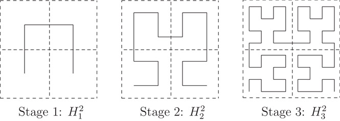
Figure 22.2The first three stages of a 2-dimensional Hilbert curve.

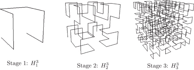
Figure 22.3The first three stages of a 3-dimensional Hilbert curve.

Each grid vertex is assigned a Hilbert value, which is an integer that corresponds to its position along the curve. For instance, in $H_{2}^{2}$ $H_{2}^{2}$ , (0, 0) and (1, 2) have Hilbert values 0 and 7, respectively. This assignment is easily extended to rectangles, in which case the Hilbert value of the grid point closest to the rectangle center is assigned. Algorithms for computing the position of a point along a space filling curve are given in References 33–35.

The structure of the R-tree is modified as follows. Leaf nodes remain the same. Each entry of an internal node now has the form (r, p, v), where r and p have the same interpretation as before, and v is the largest Hilbert value of all data items stored in the subtree with root p. This assignment results in update algorithms that are similar to those used for B⁺-trees. In particular, it is straightforward to implement an effective policy for deferred splitting which reduces the number of splits needed while performing insertions. The authors propose the following policy, which they call s-to-(s + 1) splitting. When a node overflows, an attempt is first made to shift entries laterally to s − 1 sibling nodes at the same level. An actual split occurs only if the additional entry cannot be accommodated by shifting, because the s − 1 siblings are already full. When this happens a new node is created and the sB + 1 entries are distributed among the s + 1 nodes. Because entries at the leaves are sorted by Hilbert value, bounding boxes of leaves tend to have small area and perimeter, and node utilization is high. Notice that there is a clear trade-off between node utilization and insertion complexity (which increases as s increases). The case s = 1 corresponds to the regular split policy used in the original R-tree, that is, split whenever a node overflows.

A sample tree with 5 data rectangles is shown in Figure 22.4. There are two leaf nodes and one internal node (the root). The pointer entries of the internal node are represented by arrows. Each input rectangle has been annotated with its Hilbert value. In reality, the corners of the rectangles would fall on grid vertices. They have been made smaller in order to make the figure more readable. Inserting a new rectangle whose center has Hilbert value 17 would cause an overflow in r. With deferred splitting, a split is not necessary. Instead, the new rectangle would be accommodated in r after shifting rectangle c (with Hilbert value 28) to its sibling s.

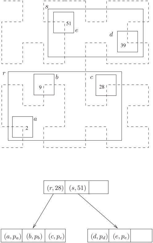
Figure 22.4A Hilbert R-tree with B = 3.

The authors report improvements of up to 28% in performance over R^*-trees and recommend using 2-to-3 splitting which results in an average node utilization of 82.2%.

In practice, one does not store or compute all bit values on the hypothetical grid. Let β be the number of bits required to describe one coordinate. Storing the Hilbert value of a d-dimensional point requires dβ bits of storage, which may be larger than the size of native machine integers. It is possible to compare the Hilbert values of two points without storing the values explicitly. Conceptually, the process computes bit positions, one at a time, until discrimination is possible. Consider the case of 2-d and notice that the first bit of the x- and y-coordinates of a point determine which quadrant contains it. Successive bits determine which successively smaller sub-quadrants contain the point. When two center points (x1, y1) and (x2, y2) need to be compared, the bits of each coordinate are examined until it can be determined that one of the points lies in a different sub-quadrant than the other (one can use the sense and rotation tables described in Reference 25 to accomplish this task). The information gathered is used to decide which point is closer to the origin (along the Hilbert Curve).

22.3.3Bulk Loading

There are applications where the data is static, or does not change very frequently. Even if the data is dynamic, it may happen that an index needs to be constructed for a large data set which is available a priori. In these circumstances, building an R-tree by inserting one object at a time has several disadvantages: (a) high load time, (b) sub-optimal space utilization, and, most important, (c) poor R-tree structure requiring the retrieval of a large number of nodes in order to satisfy a query. As discussed in the previous section, other dynamic algorithms [23,31] improve the quality of the R-tree, but still are not competitive with regard to query time when compared to loading algorithms that are allowed to pre-process the data to be stored. When done properly, preprocessing results in R-trees with nearly 100% space utilization and improved query times (due to the fact that fewer nodes need to be accessed while performing a query). Such packing algorithms were first proposed by Roussopoulos [27] and later by Kamel and Faloutsos [25], and Leutenegger et al. [26]. An approach that is intermediary between inserting a tuple at a time and constructing the entire tree by bulk loading is followed by [36], where an entire batch of input values is processed by partitioning the input into clusters and then inserting R-trees for the clusters into the existing R-tree.

The general approach to bulk loading an R-tree is similar to building a B-tree from a collection of keys by creating the leaf level first and then creating each successively higher level until the root node is created. The general approach is outlined below.

General Algorithm:

1.Sort the n rectangles and partition them into ⌈n/B⌉ consecutive groups of B rectangles. Each group of B rectangles is eventually placed in the same leaf level node. Note that the last group may contain fewer than B rectangles.

2.Load the ⌈n/B⌉ groups of rectangles into nodes and output the (MBR, address) for each leaf level node into a temporary file. The addresses are used as the child pointer fields for the nodes of the next higher level.

3.Recursively pack these MBRs into nodes at the next level, proceeding upwards, until the root node is created.

The three algorithms differ only in how the rectangles are sorted at each level. These differences are described below.

1.Nearest-X (NX):

This algorithm was proposed in Reference 27. The rectangles are sorted by the x-coordinate of a designated point such as the center. Once sorted, the rectangles are packed into nodes, in groups of size B, using this ordering. While our description is in terms of x, a different coordinate can clearly be used.

2.Hilbert Sort (HS):

The algorithm of [25] orders the rectangles using the Hilbert space filling curve. The center points of the rectangles are sorted based on their distance from the origin, measured along the curve. This process determines the order in which the rectangles are placed into the nodes of the R-Tree.

3.Sort-Tile-Recursive (STR):

STR [26] is best described recursively with d = 2 providing the base case. (The case d = 1 is already handled well by regular B-trees.) Accordingly, we first consider a set of rectangles in the plane. The basic idea is to “tile” the data space using $\sqrt{n / B}$ $\sqrt{n / B}$ vertical slices so that each slice contains enough rectangles to pack roughly $\sqrt{n / B}$ $\sqrt{n / B}$ nodes. Once again we assume coordinates are for the center points of the rectangles. Determine the number of leaf level pages P = ⌈n/B⌉ and let $S = ⌈ \sqrt{P} ⌉$ $S = ⌈ \sqrt{P} ⌉$ . Sort the rectangles by x-coordinate and partition them into S vertical slices. A slice consists of a run of S · B consecutive rectangles from the sorted list. Note that the last slice may contain fewer than S · B rectangles. Now sort the rectangles of each slice by y-coordinate and pack them into nodes by grouping them into runs of length B (the first B rectangles into the first node, the next n into the second node, and so on).

The case d > 2 is is a simple generalization of the approach described above. First, sort the hyper-rectangles according to the first coordinate of their center. Then divide the input set into $S = ⌈ P^{\frac{1}{d}} ⌉$ $S = ⌈ P^{\frac{1}{d}} ⌉$ slabs, where a slab consists of a run of $B \cdot ⌈ P^{\frac{d - 1}{d}} ⌉$ $B \cdot ⌈ P^{\frac{d - 1}{d}} ⌉$ consecutive hyper-rectangles from the sorted list. Each slab is now processed recursively using the remaining d − 1 coordinates (i.e., treated as a (d − 1)-dimensional data set).

Figure 22.5 illustrates the results from packing a set of segments from a Tiger file corresponding to the city of Long Beach. The figure shows the resultant leaf level MBRs for the same data set for each of the three algorithms using a value of B = 100 to bulk load the trees.

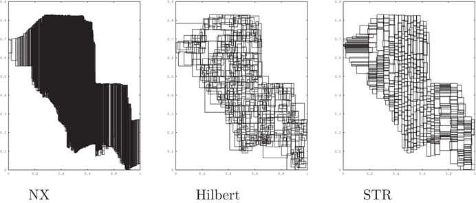
Figure 22.5Leaf level nodes for three packing algorithms.

As reported in Reference 26, both Hilbert and STR significantly outperform NX packing on all types of data except point data, where STR and NX perform similarly. For tests conducted with both synthetic and actual data sets, STR outperformed Hilbert on all but one set, by factors of up to 40%. In one instance (VLSI data), Hilbert packing performed up to 10% faster. As expected, these differences decrease rapidly as the query size increases.

22.4Advanced Operations

Even though R-trees were originally designed to perform intersections queries, it did not take long before R-trees were being used for other types of operations, such as nearest neighbor, both simple [37–39] and constrained to a range [40], reverse nearest neighbor [41–43], regular and bichromatic closest pairs [44–46], incremental nearest neighbors [38], topological queries [47], spatial joins [48–56] and distance joins [45,57]. Some of the proposals work on an ordinary R-tree while others require that the tree be modified or augmented in various ways. Because of space limitations we concentrate our attention on two problems: nearest neighbors and spatial joins.

22.4.1Nearest Neighbor Queries

We discuss the problem of finding the input object closest to an arbitrary query point Q. We assume the standard Euclidean metric, that is, if a = (a1, …, a_d) and b = (b1, …, b_d) are arbitrary points then $dist (a, b) = (\sum_{i = 1}^{d} (a_{i} - b_{i})^{2})^{1 / 2}$ $dist (a, b) = (\sum_{i = 1}^{d} (a_{i} - b_{i})^{2})^{1 / 2}$ . For a general object O, such as a rectangle or polygon, we define dist(Q, O) = min_p∈Odist(Q, p) (Figure 22.6).

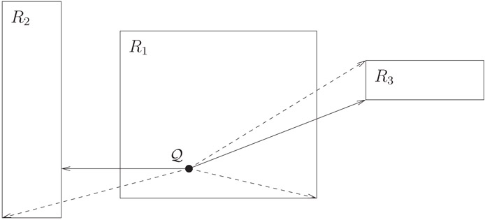
Figure 22.6Illustration of mindist (solid) and minmaxdist (dashed) for three rectangles. Notice that mindist(Q, R1) = 0 because Q ∈ R1.

The first proposal to solve this problem using R-trees is from [39]. Roussopoulos et al. define two bounding functions of Q and an arbitrary rectangle r:

mindist(Q, r) = dist(Q, r), the distance from Q to the closest point in r.

$minmaxdist (Q, r) = min_{f} max_{p \in f} (dist (Q, p)$ $minmaxdist (Q, r) = min_{f} max_{p \in f} (dist (Q, p)$ , where f ranges over all (d − 1)-dimensional facets of r.

Notice that mindist(Q, r) = 0 if Q is inside r and that for any object or rectangle s that is a descendant of r, mindist(Q, r) ≤ dist(Q, s) ≤ minmaxdist(Q, r). This last fact follows from the fact that each of the facets of r must share a point with at least one input object, but this object can be as far as possible within an incident face. Thus, the bounding functions serve as optimistic and pessimistic estimates of the distance from Q to the nearest object inside r.

The following properties of the bounding functions readily follow:

P1 For any object or MBR r and MBR s, if mindist(Q, r) > minmaxdist(Q, s) then r cannot be or contain the nearest neighbor of Q.

P2 For any MBR r and object s, if mindist(Q, r) > dist(Q, s) then r cannot contain the nearest neighbor of Q.

The authors describe a branch-and-bound algorithm that performs a depth-first traversal of the tree and keeps track of the best distance so far. The two properties above are used to identify and prune branches that are guaranteed not to contain the answer. For each call the algorithm keeps a list of active nodes, that is, nodes that tentatively need to be explored in search of a better estimate. No node of the list is explored until the subtrees corresponding to nodes appearing earlier in the active list have been processed or pruned. Thus, a sorting policy to determine the order in which rectangles stored in a node are processed is also required. In practice one would like to examine first those nodes that lower the best distance estimate as quickly as possible, but this order is difficult to determine a priori. Two criteria considered include sorting by mindist and by minmaxdist. Experimental results suggest that sorting by mindist results in slightly better performance. The algorithm is summarized in Figure 22.7. Global variable bestDistance stores the estimate of the distance to the nearest neighbor. The initial call uses the query and root of the tree as arguments.

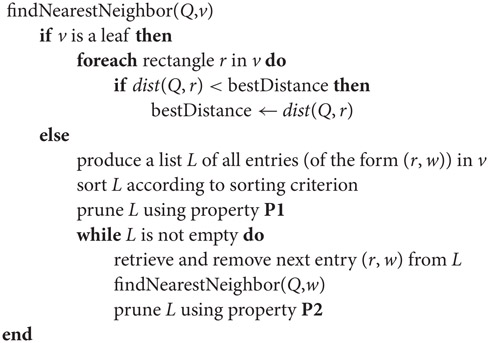
Figure 22.7Nearest neighbor algorithm of [39].

A simple modification to the above algorithm allows [39] to report the k > 1 nearest neighbors of Q. All is needed is to keep track of the best k distances encountered so far and to perform the pruning with respect to the k-th best.

Cheung and Fu [37] show that pruning based on P1 is not necessary and do away with computing minmaxdist altogether. They simplify the algorithm by pruning with P2 exclusively, and by rearranging the code so that the pruning step occurs before, and not after, each recursive call.

Hjaltason and Samet [45] also describe an algorithm that avoids using P1. Furthermore, unlike [39] which keeps a local list of active entries for each recursive call, their algorithm uses a global priority queue of active entries sorted by the optimistic distance from Q to that entry. This modification minimizes the number of R-tree nodes retrieved and results in an incremental algorithm, that is, one that reports answers in increasing order of distance, a desirable characteristic when the value of k is not known a priori.

22.4.2Spatial Joins

We consider the problem of calculating the intersection of two sets R = {r1, r2, …, r_n} and S = {s1, s2, …, s_m} of spatial objects. The spatial join, R ⋈ S, is the set of all pairs (r_i, s_j) such that r_i ∩ s_j ≠ ∅. The join of two spatial data sets is a useful and common operation. Consider, for example, the rivers and roads of a region, both represented using line segments. The spatial join of the river and road data sets yields the set of likely bridge locations. If the subset of river segments whose level is above a given threshold has been previously selected, the same spatial join now computes likely locations for road flooding.

Methods to compute spatial joins without R-trees exist but are not covered in this chapter. We consider the case where R-trees have been constructed for one or both data sets and hence can be used to facilitate the join computation. Unless otherwise stated, we will assume that the r_i’s and s_j’s refer to the MBRs enclosing the actual data objects.

In Reference 49, Brinkhoff et al. proposed the “canonical” spatial join algorithm based on R-trees. A similar join algorithm was proposed at the same time by Gunther [50]. Gunther’s algorithm is applicable for general trees and includes R-trees as a special case. In Figure 22.8 we paraphrase the algorithm of [49]. Let v1 and v2 be nodes of R-trees T1 and T2, respectively. Let E_ij, be an entry of v_i of the form $(r_{i j}, p_{i j})$ $(r_{i j}, p_{i j})$ , where r_ij and p_ij denote the MBR and child pointer, respectively. To join data sets R and S, indexed by R-trees T1 and T2, invoke the SpatialJoin algorithm in Figure 22.8, passing as arguments the roots of T1 and T2.

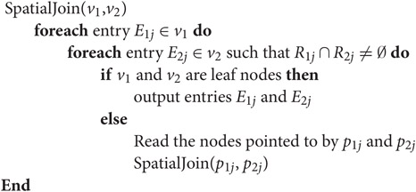
Figure 22.8Spatial join algorithm of [49] for two R-trees.

In Reference 49 the authors generalize the algorithm for the case where the two R-trees have different heights. They also improve upon the basic algorithm by reducing CPU computation and disk accesses. The CPU time is improved by reducing the number of rectangle intersection checks. One method to accomplish this is to first calculate the subset of entries within nodes v1 and v2 that intersect MBR(v1) ∩ MBR(v2), and then do full intersection tests among this subset. A second approach is to sort the entries and then use a sweep-line algorithm. In addition, the paper considers reduction of page I/O by ordering the accesses to pages so as to improve the buffer hit ratio. This is done by accessing the data in sweep-line order or Z-order.

In Reference 48 Brinkhoff et al. suggest the following 3-step approach for joining complex polygonal data sets: (1) use the R-trees and MBRs of the data sets to reduce the set to a list of potential hits; (2) use a lightweight approximation algorithm to further reduce the set, leaving in some “false positives”; (3) conduct the exact intersection tests on the remaining polygons using techniques from computational geometry (see Chapter 2 of [58], for example).

Often only one of the data sets to be joined will be indexed by an R-tree. This is the case when the DBA decides that maintaining an index is too expensive, when the data set being joined is the result of a series of non-spatial attribute selections, or for multi-step joins where intermediate results are not indexed.

To join two data sets when only one is indexed by an R-tree, Lo and Ravishankar [52] propose the idea of seeded tree join. The main idea is to use the existing R-tree to “seed” the creation of a new index, called the seeded tree, for the non-indexed data set, and then perform a join using the method of [49].

Consider the example shown in Figure 22.9 (similar to the example in Reference 52). Assume that the existing tree has four entries in the root node. The four rectangles, R1 to R4, in the left hand side represent the bounding rectangles of these entries. The dark filled squares do not belong to the existing R-tree but, rather, correspond to some of the data items in the non-indexed data set. Assuming a node capacity of four (i.e., B = 4) and using the normal insertion or loading algorithms which minimize area and perimeter, the dark rectangles would likely be grouped as shown by the dark MBRs in Figure 22.9b. A spatial join would then require that each node of each tree be joined with two nodes from the other tree, for a total of eight pairs. On the other hand, if the second R-tree was structured as show in Figure 22.9c, then each node would be joined with only one node from the other tree, for a total of four pairs. Hence, when performing a spatial join, it might be better to structure the top levels of the tree in a fashion that is sub-optimal for general window queries.

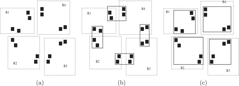
Figure 22.9Seeded Tree Example. (a) Existing R-tree and non-indexed data (dark squares); (b) Normal R-tree structure for non-indexed data; (c) Seeded structure.

The general algorithm for seeded tree creation is to copy the top few levels of the existing tree and use them as the top levels for the new tree. These top levels are called the seed levels. The entries at the lowest seed level are called “slots”. Non-indexed data items are then inserted into the seeded tree by inserting them into an R-tree that is built under the appropriate slot. In Reference 52 the authors experimentally compare three join algorithms: (1) R-tree join, where an R-tree is fist built on the non-indexed data set and then joined; (2) brute force, where the non-indexed data set is read sequentially and a region query is run against the existing R-tree for each data item in the non-indexed data set; (3) seeded tree join, where a seeded tree is built and then joined. The authors consider several variants of the seeded tree creation algorithm and compare the performance. Experimental studies show that the seeded tree method significantly reduces I/O. Note that if the entire seeded tree does not fit in memory significant I/O can occur during the building process. The authors propose to minimize this I/O by buffering runs for the slots and then building the tree for each slot during a second pass.

Another approach [51] for the one-index case is to sort the non-indexed data using the MBR lower endpoints for one of the dimensions, sort the leaf level MBRs from the existing R-tree on the same dimension, and finally join the two sorted data sets using a sweep-line algorithm. The authors analytically demonstrate that as long as the buffer size is sufficient to merge-sort efficiently, their algorithm results in less I/O than creating any type of index followed by a join. Experimental results also show a significant I/O reduction.

In Reference 56 a relational hash-based join approach is used. Although mostly hash-based, the method does need to default to R-trees in some cases. A sampled subset of R is partitioned into N buckets, R1…R_N, for some N. Each non-sampled object from R is then added to the bucket that requires the least enlargement. Set S is then partitioned in N corresponding buckets, S1…S_N by testing each object o_S of S and placing a copy of it into S_i, for each bucket R_i such that o_S ∩ R_i ≠ ∅. If an object in S does not intersect any of the R_i buckets the object is discarded. The bucket pairs (R_i, S_i) are then read into memory and pairwise joined. If a bucket pair is too large to fit in memory, an R-tree index is built for one of the two buckets and an index-loop join is used.

In References 53 and 55 a method that combines the seeded tree and the hash-join approach is proposed. The proposed method, slot index spatial join, chooses a level from the existing tree and uses the MBRs of the entries as the buckets for the hashing. The chosen level is determined by the number of entries at that level and the number of buffer pages available for the bucket joining algorithm. Since R-trees have a wide fan out, the optimal number of buckets to use usually falls between level sizes. The paper considers several heuristics for combining MBRs from the next level down to tune the number of buckets. Overall performance is shown to be better than all previously existing methods in all but a few cases.

A method to join multiple spatial relations together is discussed in Reference 53 and 54. The authors propose a multi-way join algorithm called synchronous traversal and develop cost models to use for query optimization. They consider using only pairwise joins, only the synchronous traversal method, and combinations of the two approaches. They show that, in general, a combination of the two results in the best performance.

The concept of spatial join has been further generalized to distance joins, where a distance based ordering of a subset of the Cartesian product of the two sets is returned. In References 45 and 57, distance join algorithms using R-trees are proposed.

22.5Analytical Models

Analytical models of R-trees provide performance estimates based on the assumptions of the model. Such models can be useful for gaining insight, comparing algorithms, and for query optimization.

Early analytical models for range queries were proposed by Kamel and Faloutsos [25], and Pagel et al. [59]. The models are similar and use the MBRs of all nodes in the tree as inputs to the model. They derive the probability that Q intersects a given MBR, and use this estimate to compute the expected number of MBRs intersected by Q. In References 60 and 61 the basic model was modified to correct for an error that may arise for MBRs near the boundary of the query sample space. In order to do this, [61] assumes that all queries fall completely within the data space. The changes necessary to handle different sample spaces are straightforward.

The models provide good insight into the problem, especially by establishing a quantitative relationship between performance and the total area and perimeter of MBRs of the tree nodes. We describe the model as presented in Reference 61.

Consider a 2-dimensional data set consisting of rectangles to be stored in an R-tree T with h + 1 levels, labeled 0 through h. Assume all input rectangles have been normalized to fit within the unit square U = [0, 1] × [0, 1]. Queries are rectangles Q of size q_x × q_y. (A point query corresponds to the case q_x = q_y = 0.) Initially assume that queries are uniformly distributed over the unit square. Although this description concentrates on 2-d, generalizations to higher dimensions are straightforward.

Assume the following notation:

m_i = number of nodes at the i th level of T

m = Total number nodes in T, that is, $\sum_{i = 0}^{h} m_{i}$ $\sum_{i = 0}^{h} m_{i}$

R_ij = jth rectangle at the ith level of T

X_ij = x-extent (width) of R_ij

Y_ij = y-extent (height) of R_ij

A_ij = area of R_ij, that is, $A_{i j} = X_{i j} \cdot Y_{i j}$ $A_{i j} = X_{i j} \cdot Y_{i j}$

$A_{i j}^{Q}$ $A_{i j}^{Q}$ = probability that R_ij is accessed by query Q

B_ij = number of accesses to R_ij

$A$ $A$ = Sum of the areas of all MBRs in T

L_x = Sum of the x-extents of all MBRs in T

L_y = Sum of the y-extents of all MBRs in T

N = number of queries performed so far

N^* = expected number of queries required to fill the buffer

β = buffer size

D(N) = number of distinct nodes (at all levels) accessed in N queries

$E_{T}^{P} (q_{x}, q_{y})$ $E_{T}^{P} (q_{x}, q_{y})$ = expected number of nodes (buffer resident or not) of T accessed while performing a query of size q_x × q_y

$E_{T}^{D} (q_{x}, q_{y})$ $E_{T}^{D} (q_{x}, q_{y})$ = expected number of disk accesses while performing a query of size q_x × q_y

The authors of [25,59] assume that performance is measured by the number of nodes accessed (independent of buffering). They observe that for uniform point queries the probability of accessing R_ij is just the area of R_ij, namely, A_ij. They point out that the level of T in which R_ij resides is immaterial as all rectangles containing Q (and only those) need to be retrieved. Accordingly, for a point query, the expected number of nodes retrieved as derived in Reference 25 is the sum of node areas^*:

$E_{T}^{P} (0, 0) = \sum_{i = 0}^{h} \sum_{j = 1}^{m_{i}} A_{i j} = A$ $E_{T}^{P} (0, 0) = \sum_{i = 0}^{h} \sum_{j = 1}^{m_{i}} A_{i j} = A$	(22.1)

which is the sum of the areas of all rectangles (both leaf level MBRs as well as MBRs of internal nodes).

We now turn our attention to region queries. Let 〈(a, b), (c, d)〉 denote an axis-parallel rectangle with bottom left and top right corners (a, b) and (c, d), respectively. Consider a rectangular query $Q = 〈 Q_{b l}, Q_{t r} 〉$ $Q = 〈 Q_{b l}, Q_{t r} 〉$ of size q_x × q_y. Q intersects R = 〈(a, b), (c, d)〉 if and only if Q_tr (the top right corner of Q) is inside the extended rectangle R′ = 〈(a, b), (c + q_x, d + q_y)〉, as illustrated in Figure 22.10.

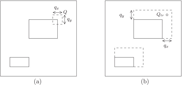
Figure 22.10(a) Two data rectangles and region query Q. (b) Corresponding extended rectangles and equivalent point query Q_tr.

Kamel and Faloutsos infer that the probability of accessing R while performing Q is the area of R′, as the region query Q is equivalent to a point query Q_tr where all rectangles in T have been extended as outlined above. Thus, the expected number of nodes retrieved (as derived in Reference 25) is:

\begin{aligned} E_{T}^{P} (q_{x}, q_{y}) & = \sum_{i = 0}^{h} \sum_{j = 1}^{m_{i}} (X_{i j} + q_{x}) (Y_{i j} + q_{y}) \\ = \sum_{i = 0}^{h} \sum_{j = 1}^{m_{i}} X_{i j} Y_{i j} + q_{x} \sum_{i = 0}^{h} \sum_{j = 1}^{m_{i}} Y_{i j} + q_{y} \sum_{i = 0}^{h} \sum_{j = 1}^{m_{i}} X_{i j} + m q_{x} q_{y} \\ = A + q_{x} L_{y} + q_{y} L_{x} + m q_{x} q_{y} \end{aligned}

$\begin{aligned} E_{T}^{P} (q_{x}, q_{y}) & = \sum_{i = 0}^{h} \sum_{j = 1}^{m_{i}} (X_{i j} + q_{x}) (Y_{i j} + q_{y}) \\ = \sum_{i = 0}^{h} \sum_{j = 1}^{m_{i}} X_{i j} Y_{i j} + q_{x} \sum_{i = 0}^{h} \sum_{j = 1}^{m_{i}} Y_{i j} + q_{y} \sum_{i = 0}^{h} \sum_{j = 1}^{m_{i}} X_{i j} + m q_{x} q_{y} \\ = A + q_{x} L_{y} + q_{y} L_{x} + m q_{x} q_{y} \end{aligned}$

(22.2)

Equation 22.3 illustrates the fact that a good insertion/loading algorithm should cluster rectangles so as to minimize both the total area and total perimeter of the MBRs of all nodes. For point queries, on the other hand, q_x = q_y = 0, and minimizing the total area is enough.

In Reference 61 the model of [25] was modified to handle query windows that fall partially outside the data space as well as data rectangles close to the boundary of the data space, as suggested by Six et al. [59]. Specifically:

1.For uniformly distributed rectangular queries of size q_x × q_y the top right corner of the query region Q, cannot be an arbitrary point inside the unit square if the entire query region is to fit within the unit square. For example, if q_x = q_y = 0.3, a query such as Q1 in Figure 22.11a should not be allowed. Rather, Q_tr must be inside the box U′ = [q_x, 1] × [q_y, 1].

2.The probability of accessing a rectangle R = 〈(a, b), (c, d)〉 is not always the area of R′ = 〈(a, b), (c + q_x, d + q_y)〉 as this value can be bigger than one. For example, in Figure 22.11b, the probability that a query of size 0.8 × 0.8 accesses rectangle R1 should not be 1.1·1.1 = 1.21, which is the area of the extended rectangle $R_{1}^{'}$ $R_{1}^{'}$ , obtained by applying the original formula. Rather, the access probability is the percentage of U′ covered by the rectangle R′ ∩ U′.

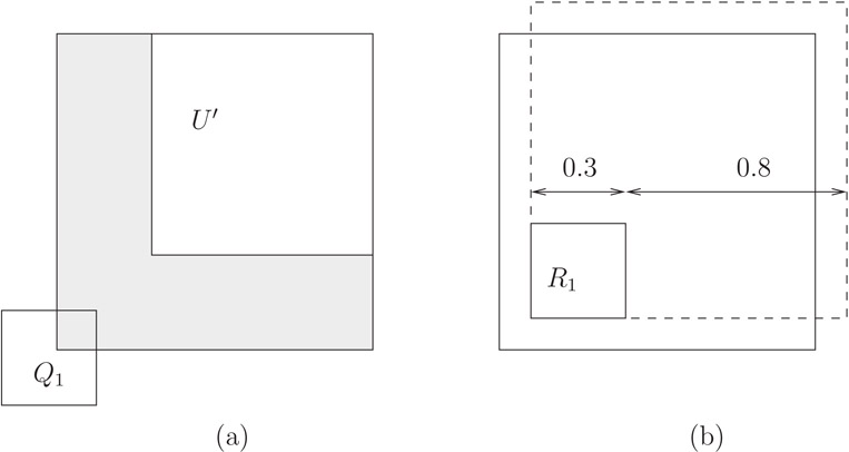
Figure 22.11The domain of Q_tr for a query of size 0.3 × 0.3 is U′ (area not shaded).

Thus, we change the probability of accessing rectangle i of level j to:

$\begin{aligned} A_{i, j}^{Q} & = \frac{area (R^{'} \cap U^{'})}{area (U^{'})} \\ = \frac{C \cdot D}{(1 - q_{x}) (1 - q_{y})} \end{aligned}$ $\begin{aligned} A_{i, j}^{Q} & = \frac{area (R^{'} \cap U^{'})}{area (U^{'})} \\ = \frac{C \cdot D}{(1 - q_{x}) (1 - q_{y})} \end{aligned}$	(22.3)

where C = [min(1, c + q_x) − max(a, q_x)] and D = [min(1, d + q_y) − max(b, q_y)].

In Reference 62 the R-tree model was expanded to take into account the distribution of the input data. Specifically, rather than being uniformly distributed, the query regions were assumed to be distributed according to the input data distribution.

The above models do not consider the impact of the buffer. In Reference 62 a buffer model is integrated with the query model. Specifically, under uniformly distributed point queries, the probability of accessing rectangle R_ij while performing a query is A_ij. Accordingly, the probability that R_ij is not accessed during the next N queries is $P [B_{i j} = 0 | N] = (1 - A_{i j})^{N}$ $P [B_{i j} = 0 | N] = (1 - A_{i j})^{N}$ . Thus, $P [B_{i j} \geq 1 | N] = 1 - (1 - A_{i j})^{N}$ $P [B_{i j} \geq 1 | N] = 1 - (1 - A_{i j})^{N}$ and the expected number of distinct nodes accessed in N queries is,

$D (N) = \sum_{i = 0}^{h} \sum_{j = 1}^{m_{i}} P [B_{i j} \geq 1 \| N] = m - \sum_{i = 0}^{h} \sum_{j = 1}^{m_{i}} (1 - A_{i j})^{N}$ $D (N) = \sum_{i = 0}^{h} \sum_{j = 1}^{m_{i}} P [B_{i j} \geq 1 \| N] = m - \sum_{i = 0}^{h} \sum_{j = 1}^{m_{i}} (1 - A_{i j})^{N}$	(22.4)

Note that D(0) = 0 < β and $D (1) = A$ $D (1) = A$ (which may or may not be bigger than β). The buffer, which is initially empty, first becomes full after performing N^* queries, where N^* is the smallest integer that satisfies D(N^*) ≥ β. The value of N^* can be determined by a simple binary search.

While the buffer is not full the probability that R_ij is in the buffer is equal to P[B_ij ≥ 1]. The probability that a random query requires a disk access for R_ij is $A_{i j} \cdot P [B_{i j} = 0]$ $A_{i j} \cdot P [B_{i j} = 0]$ . Since the steady state buffer hit probability is approximately the same as the buffer hit probability after N^* queries, the expected number of disk accesses for a point query at steady state is

$\sum_{i = 0}^{h} \sum_{j = 1}^{m_{i}} A_{i j} \cdot P [B_{i j} = 0 \| N^{}] = \sum_{i = 0}^{h} \sum_{j = 1}^{m_{i}} A_{i j} \cdot (1 - A_{i j})^{N^{}}$ $\sum_{i = 0}^{h} \sum_{j = 1}^{m_{i}} A_{i j} \cdot P [B_{i j} = 0 \| N^{}] = \sum_{i = 0}^{h} \sum_{j = 1}^{m_{i}} A_{i j} \cdot (1 - A_{i j})^{N^{}}$	(22.5)

The above derivation also holds for region queries provided that $A_{i j}^{Q}$ $A_{i j}^{Q}$ is used instead of A_ij, that is:

E_{T}^{D} (q_{x}, q_{y}) = \sum_{i = 0}^{h} \sum_{j = 1}^{m_{i}} A_{i j}^{Q} \cdot {(1 - A_{i j}^{Q})}^{N^{*}}

$E_{T}^{D} (q_{x}, q_{y}) = \sum_{i = 0}^{h} \sum_{j = 1}^{m_{i}} A_{i j}^{Q} \cdot {(1 - A_{i j}^{Q})}^{N^{*}}$

In Reference 61 the authors compare the model to simulation and explore the I/O impact of pinning the top levels of an R-tree into the buffer.

Other analytical models include the following. Theodoridis and Sellis [63] provide a fully analytical model that does not require the R-tree MBRs as input. In Reference 64, a technique is developed for analyzing R-tree performance with skewed data distributions. The technique uses the concept of fractal dimension to characterize the data set and resultant R-tree performance. Analysis has also been used for estimating the performance of R-tree based spatial joins [65,66] and nearest neighbor queries [67,68].

Acknowledgment

This work was supported in part by the National Science Foundation under Grants IRI-9610240 and DMS-0107628.

References

1.D. Comer. The ubiquitous B-tree. ACM Computing Surveys, 11(2):121–137, 1979.

2.A. Guttman. R-trees: A dynamic index structure for spatial searching. In Proc. ACM SIGMOD, pages 47–57, June 1984.

3.T. Brinkhoff, H.-P. Kriegel, and B. Seeger. Parallel processing of spatial joins using R-trees. In Proc. 12th International Conference on Data Engineering (ICDE), pages 258–265, 1996.

4.I. Kamel and C. Faloutsos. Parallel R-trees. In Proc. ACM SIGMOD, pages 195–204, April 1992.

5.A. Papadopoulos and Y. Manolopoulos. Similarity query processing using disk arrays. In Proc. ACM SIGMOD, pages 225–236, 1998. parallel NN using R-trees.

6.B. Schnitzer and S.T. Leutenegger. Master-client R-trees: A new parallel R-tree architecture. In Proc. Conference of Scientific and Statistical Database Systems (SSDBM), pages 68–77, 1999.

7.S. Berchtold, D. Keim, and H.-P. Kriegel. The X-tree: An index structure for high-dimensional data. In Proc. 22nd International Conference on Very Large Databases (VLDB), pages 28–39, 1996.

8.N. Katayama and S. Satoh. The SR-tree: An index structure for high-dimensional nearest neighbor queries. In Proc. ACM SIGMOD, pages 369–380, 1997.

9.D. White and R. Jain. Similarity indexing: Algorithms and performance. In Proc. SPIE Storage and Retrieval for Still Image and Video Databases IV, volume 2670, pages 62–73, 1996.

10.G. Kollios, V.J. Tsotras, D. Gunopulos, A. Delis, and M. Hadjieleftheriou. Indexing animated objects using spatiotemporal access methods. IEEE Transactions on Knowledge and Data Engineering, 13(5):758–777, 2001.

11.D. Pfoser, C.S. Jensen, and Y. Theodoridis. Novel approaches in query processing for moving object trajectories. In Proc. 26th International Conference on Very Large Databases (VLDB), pages 395–406, 2000.

12.C.M. Procopiuc, P.K. Agarwal, and S. Har-Peled. Star-tree: An efficient self-adjusting index for moving objects. In Proc. 4th Workshop on Algorithm Engineering and Experiments (ALENEX), pages 178–193, 2002.

13.S. Saltenis and C. Jensen. Indexing of now-relative spatio-bitemporal data. The VLDB Journal, 11(1):1–16, 2002.

14.S. Saltenis, C. Jensen, S. Leutenegger, and M.A. Lopez. Indexing the positions of continuously moving points. In Proc. ACM SIGMOD, pages 331–342, May 2000.

15.Y. Tao and D. Papadias. MV3R-tree: A spatio-temporal access method for timestamp and interval queries. In Proc. 27th International Conference on Very Large Databases (VLDB), pages 431–440, 2001.

16.Y. Tao, D. Papadias, and J. Sun. The TPR^*-tree: An optimized spatio-temporal access method for predictive queries. In Proc. International Conference on Very Large Databases (VLDB), pages 790–801, 2003.

17.M. Kornacker and D. Banks. High-concurrency locking in R-trees. In Proc. International Conference on Very Large DataBases (VLDB), pages 134–145, 1995.

18.V. Ng and T. Kameda. Concurrent access to R-trees. In Proc. SSD, pages 142–161, 1993.

19.B.-U. Pagel, H.-W. Six, and M. Winter. Window query-optimal clustering of spatial objects. In Proc. 14th ACM Symposium on Principles of Database Systems (PODS), pages 86–94, 1995.

20.C.H. Ang and T.C. Tan. New linear node splitting algorithm for R-trees. In Advances in Spatial Databases, 5th International Symposium (SSD), volume 1262 of Lecture Notes in Computer Science, pages 339–349. Springer, 1997.

21.B. Becker, P. G. Franciosa, S. Gschwind, S. Leonardi, T. Ohler, and P. Widmayer. Enclosing a set of objects by two minimum area rectangles. Journal of Algorithms, 21(3):520–541, 1996.

22.Y. Garcia, M.A. Lopez, and S.T. Leutenegger. On optimal node splitting for R-trees. In Proc. International Conference on Very Large Databases (VLDB), pages 334–344, August 1998.

23.N. Beckmann, H.P. Kriegel, R. Schneider, and B. Seeger. The R^⋆-tree: An efficient and robust access method for points and rectangles. In Proc. ACM SIGMOD, pages 323–331, May 1990.

24.I. Kamel and C. Faloutsos. Hilbert R-tree: An improved R-tree using fractals. In Proc. International Conference on Very Large Databases (VLDB), pages 500–509, September 1994.

25.I. Kamel and C. Faloutsos. On packing R-trees. In Proc. 2nd International Conference on Information and Knowledge Management (CIKM), pages 490–499, Washington D.C., November 1993.

26.S.T. Leutenegger, M.A. Lopez, and J.M. Edgington. STR: A simple and efficient algorithm for R-tree packing. In Proc. 14th International Conference on Data Engineering (ICDE), pages 497–506, 1997.

27.N. Roussopoulos and D. Leifker. Direct spatial search on pictorial databases using packed R-trees. In Proc. ACM SIGMOD, pages 17–31, Austin, Texas, May 1985.

28.M. de Berg, J. Gudmundsson, M. Hammar, and M. Overmars. On R-trees with low query complexity. Computational geometry: Theory of Applications, 24(3):179–195, 2003.

29.Y. Garcia, M.A. Lopez, and S.T. Leutenegger. Post-optimization and incremental refinement of R-trees. In Proc. 7th International Symposium on Advances in Geographic Information Systems (ACM GIS), pages 91–96, ACM, 1999.

30.T. Schreck and Z. Chen. Branch grafting method for R-tree implementation. Journal of Systems and Software, 53:83–93, 2000.

31.T. Sellis, N. Roussopoulos, and C. Faloutsos. The R⁺ tree: A dynamic index for multidimensional objects. In Proc. 13th International Conference on Very Large Databases (VLDB), pages 507–518, September 1987.

32.H. Sagan. Space-filling curves. Springer-Verlag, New York, 1994.

33.T. Bially. Space-filling curves: Their generation and their application to bandwidth reduction. IEEE Transactions on Information Theory, IT-15(6):658–664, 1969.

34.A.R. Butz. Alternative algorithm for Hilbert’s space-filling curve. IEEE Transactions on Computers, C-20:424–426, 1971.

35.K. Sevcik and N. Koudas. Filter trees for managing spatial data over a range of size granularities. Technical Report CSRI-TR-333, Computer Systems Research Institute, University of Toronto, October 1995.

36.R. Choubey, L. Chen, and E.A. Rundensteiner. GBI: A generalized R-tree bulk-insertion strategy. In Symposium on Large Spatial Databases, pages 91–108, 1999.

37.K.L. Cheung and A.W.-C. Fu. Enhanced nearest neighbour search on the R-tree. SIGMOD Record, 27(3):16–21, 1998.

38.G.R. Hjaltason and H. Samet. Distance browsing in spatial databases. ACM Transactions on Database Systems, 24(2):265–318, 1999.

39.N. Roussopoulos, S. Kelley, and F. Vincent. Nearest neighbor queries. In Proc. ACM SIGMOD, pages 71–79, May 1995.

40.H. Ferhatosmanoglu, I. Stanoi, D. Agrawal, and A. El Abbadi. Constrained nearest neighbor queries. Lecture Notes in Computer Science, 2121:257–278, 2001.

41.F. Korn and S. Muthukrishnan. Influence sets based on reverse nearest neighbor queries. In Proc. ACM SIGMOD, pages 201–212, 2000.

42.I. Stanoi, D. Agrawal, and A. El Abbadi. Reverse nearest neighbor queries for dynamic databases. In ACM SIGMOD Workshop on Research Issues in Data Mining and Knowledge Discovery, pages 44–53, 2000.

43.C. Yang and K.-I. Lin. An index structure for efficient reverse nearest neighbor queries. In Proc. International Conference on Data Engineering (ICDE), pages 485–492, 2001.

44.A. Corral, Y. Manolopoulos, Y. Theodoridis, and M. Vassilakopoulos. Closest pair queries in spatial databases. In Proc. ACM SIGMOD, pages 189–200, 2000.

45.G.R. Hjaltason, and H. Samet. Incremental distance join algorithms for spatial databases. In Proc. ACM SIGMOD, pages 237–248, 1998.

46.J. Shan, D. Zhang, and B. Salzberg. On spatia-range closest-pair queries. In Proc. 8th International Symposium on Spatial and Temporal Databases (SSTD), pages 252–269, 2003.

47.D. Papadias, T. Sellis, Y. Theodoridis, and M. Egenhofer. Topological relations in the world of minimum bounding rectangles: A study with R-trees. In Proc. ACM SIGMOD, pages 92–103, 1995.

48.T. Brinkhoff, H.-P. Kriegel, R. Schneider, and B. Seeger. Multi-step processing of spatial joins. In Proc. ACM SIGMOD, pages 197–208, 1994.

49.T. Brinkhoff, H.-P. Kriegel, and B. Seeger. Efficient processing of spatial joins using R-trees. In Proc. ACM SIGMOD, pages 237–246, 1993.

50.O. Gunther. Efficient computation of spatial joins. In Proc. International Conference on Data Engineering (ICDE), pages 50–59, 1993.

51.C. Gurret and P. Rigaux. The sort/sweep algorithm: A new method for R-tree based spatial joins. In Proc. SSDBM, pages 153–165, 2002.

52.M-L. Lo and C.V. Ravishankar. Spatial joins using seeded trees. In Proc. ACM SIGMOD, pages 209–220, 1994.

53.N. Mamoulis and D. Papadias. Integration of spatial join algorithms for processing multiple inputs. In Proc. ACM SIGMOD, pages 1–12, Philadelphia, Pennsylvania, June 1999.

54.N. Mamoulis and D. Papadias. Multiway spatial joins. ACM Transactions on Database systems, 26(4):424–475, 2001.

55.N. Mamoulis and D. Papadias. Slot index spatial join. IEEE Transactions on Knowledge and Data Engineering, 15(1):1–21, 2003.

56.J.M. Patel and D.J. DeWitt. Partition based spatial-merge join. In Proc. ACM SIGMOD, pages 259–270, Montreal, Quebec, June 1996.

57.H. Shin, B. Moon, and S. Lee. Adaptive multi-stage distance join processing. In Proc. ACM SIGMOD, pages 343–354, 2000.

58.M. de Berg, O. Cheong, M. van Kreveld, and M. Overmars. Computational Geometry: Algorithms and Applications. Springer-Verlag, Berlin, Heidelberg, 3rd edition, 2008.

59.B-U. Pagel, H-W. Six, H. Toben, and P. Widmayer. Towards an analysis of range query performance in spatial data structures. In Proc. ACM Symposium on Principles of Database Systems (PODS), pages 214–221, May 1993.

60.S. Berchtold, C. Bohm, and H.-P. Kriegel. Improving the query performance of high-dimensional index structures by bulk-load operations. In Proc. 6th International Conference on Extending Database Technology, pages 216–230, 1998.

61.S.T. Leutenegger and M.A. Lopez. The effect of buffering on the performance of R-trees. In Proc. 15th International Conference on Data Engineering (ICDE), pages 164–171, 1998.

62.S.T. Leutenegger and M.A. Lopez. The effect of buffering on the performance of R-trees. IEEE Transactions on Knowledge and Data Engineering, 12(1):33–44, 2000.

63.Y. Theodoridis and T. Sellis. A model for the prediction of R-tree performance. In Proc. 8th ACM Symposium on Principles of Database Systems (PODS), pages 161–171, Montreal, Quebec, Jun 1996.

64.C. Faloutsos and I. Kamel. Beyond uniformity and independence: Analysis of R-trees using the concept of fractal dimension. In Proc. ACM Symposium on Principles of Database Systems (PODS), pages 4–13, 1994.

65.Y.-W. Huang, N. Jing, and E. A. Rundensteiner. A cost model for estimating the performance of spatial joins using R-trees. In Statistical and Scientific Database Management, pages 30–38, 1997.

66.Y. Theodoridis, E. Stefanakis, and T. K. Sellis. Efficient cost models for spatial queries using R-trees. IEEE Transactions on Knowledge and Data Engineering, 12(1):19–32, 2000.

67.A. Papadopoulos and Y. Manolopoulos. Performance of nearest neighbor queries in R-trees. In Proc. 6th International Conference on Database Theory, pages 394–408, 1997.

68.Y. Tao, J. Zhang, D. Papadias, and N. Mamoulis. An efficient cost model for optimization of nearest neighbor search in low and medium dimensional spaces. IEEE Transactions on Knowledge and Data Engineering, 16(10):1169–1184, 2004.

*This chapter has been reprinted from first edition of this Handbook, without any content updates.

*We have modified the notation of [25] to make it consistent with the notation used here.

..................Content has been hidden....................

You can't read the all page of ebook, please click here login for view all page.

Table of Contents for 22. R-Trees

Create new playlist

Sign In

Sign Up

Table of Contents for
22. R-Trees