
Approximate Geometric Query Structures*
Christian A. Duncan
Quinnipiac University
Michael T. Goodrich
University of California, Irvine
Specializeddata structures are useful for answering specific kinds of geometric queries. Such structures are tailor-made for the kinds of queries that are anticipated and even then there are cases when producing an exact answer is only slightly better than an exhaustive search. For example, Chazelle and Welzl [1] showed that triangle range queries can be solved in time using linear space but this holds only in the plane. In higher dimensions, the running times go up dramatically, so that, in general, the time needed to perform an exact simplex range query and still use small linear space is roughly Ω(n1−1/d), ignoring logarithmic factors [2]. For orthogonal range queries, efficient query processing is possible if superlinear space is allowed. For example, range trees (Chapter 19) can answer orthogonal range queries in O(logd−1n) time but use O(n logd−1n) space [3].
In this chapter, we focus instead on general-purpose data structures that can answer nearest-neighbor queries and range queries using linear space. Since the lower-bound of Chazelle [2] applies in this context, in order to get query bounds that are significantly faster than exhaustive search, we need to compromise somewhat on the exactness of our answers. That is, we will answer all queries approximately, giving responses that are within an arbitrarily small constant factor of the exact solution. As we discuss, such responses can typically be produced in logarithmic or polylogarithmic time, using linear space. Moreover, in many practical situations, a good approximate solution is often sufficient.
In recent years several interesting data structures have emerged that efficiently solve several general kinds of geometric queries approximately. We review three major classes of such structures in this chapter. The first one we discuss is a structure introduced by Arya et al. [4] for efficiently approximating nearest-neighbor queries in low-dimensional space. Their work developed a new structure known as the balanced box decomposition (BBD) tree. The BBD tree is a variant of the quadtree and octree [5] but is most closely related to the fair-split tree of Callahan and Kosaraju [6]. In Reference 7, Arya and Mount extend the structure to show that it can also answer approximate range queries. Their structure is based on the decomposition of space into “boxes” that may have a smaller box “cut out;” hence, the boxes may not be convex. The second general purpose data structure we discuss is the balanced aspect ratio (BAR) tree of Duncan et al. [8–10], which is a structure that has similar performance as the BBD tree but decomposes space into convex regions. Finally, we discuss an analysis of a type of k-d tree [11] that helps to explain why k-d trees have long been known to exhibit excellent performance bounds in practice for general geometric queries. In particular, we review a result of Dickerson et al. [8,12], which shows that one of the more common variants, the maximum-spread k-d tree, exhibits properties similar to BBD trees and BAR trees; we present efficient bounds on approximate geometric queries for this variant. Unfortunately, the bounds are not as efficient as the BBD tree or BAR tree but are comparable.
In order to discuss approximate geometric queries and the efficient structures on them without confusion, we must cover a few fundamental terms. We distinguish between general points in ℝd and points given as input to the structures.
For a given metric space ℝd, the coordinates of any point p ∈ ℝd are (p1, p2, …, pd). When necessary to avoid confusion, we refer to points given as input in a set S as data points and general points in ℝd as real points. For two points p, q ∈ ℝd, the Lm metric distance between p and q is
Although our analysis will concentrate on the Euclidean L2 metric space, the data structures mentioned in this chapter work in all of the Lm metric spaces.
In addition, we use the standard notions of (convex) regions R, rectangular boxes, hyperplanes H, and hyperspheres B. For each of these objects we define two distance values. Let P and Q be any two regions in ℝd, the minimum and maximum metric distances between P and Q are
Notice that this definition holds even if one or both regions are simply points.
Let S be a finite data set S ⊂ ℝd. For a subset S1 ⊆ S, the size of S1, written |S1|, is the number of distinct data points in S1. More importantly, for any region R ⊂ ℝd, the size is |R| = |R ∩ S|. That is, the size of a region identifies the number of data points in it. To refer to the physical size of a region, we define the outer radius as , where Br is defined as the hypersphere with radius r. The inner radius of a region is . The outer radius, therefore, identifies the smallest ball that contains the region R whereas the inner radius identifies the largest ball contained in R.
In order to discuss balanced aspect ratio, we need to define the term.
Definition 27.1
A convex region R in ℝd has aspect ratio asp(R) = OR/IR with respect to some underlying metric. For a given balancing factor α, if asp(R) ≤ α, R has balanced aspect ratio and is called an α-balanced region. Similarly, a collection of regions has balanced aspect ratio for a given factor α if each region is an α-balanced region.
For simplicity, when referring to rectangular boxes, we consider the aspect ratio as simply the ratio of the longest side to the shortest side. It is fairly easy to verify that the two definitions are equal within a constant factor. As is commonly used, we refer to regions as being either fat or skinny depending on whether their aspect ratios are balanced or not.
The class of structures that we discuss in this chapter are all derivatives of binary space partition (BSP) trees, see for example [13]. See also Chapter 21. Each node u in a BSP tree T represents both a region Ru in space and the data subset Su ⊆ S of objects, points, lying inside Ru. For simplicity, regions are considered closed and points falling on the boundary of two regions can be in either of the two regions but not both. Each leaf node in T represents a region with a constant number of data objects, points, from S. Each internal node in T has an associated cut partitioning the region into two subregions, each a child node. The root of T is associated with some bounding (rectangular box) region containing S. In general, BSP trees can store any type of object, points, lines, solids, but in our case we focus on points. Typically, the partitioning cuts used are hyperplanes resulting in convex regions. However, the BBD tree presented in Section 27.5 is slightly different and can introduce regions with a single interior hole. Therefore, we have generalized slightly to accommodate this in our definition.
Before elaborating on the structures and search algorithms used to answer certain geometric queries, let us first introduce the basic definitions of approximate nearest-neighbor, farthest-neighbor, and range queries, see [4,7,8,10,14].
Definition 27.2
Given a set S of points in ℝd, a query point q ∈ ℝd, a (connected) query region Q ⊂ ℝd, and ε > 0, we define the following queries (see Figure 27.1):
•A point p* ∈ S is a nearest neighbor of q if δ(p*, q) ≤ δ(p, q) for all p ∈ S.
•A point p* ∈ S is a farthest neighbor of q if δ(p*, q) ≥ δ(p, q) for all p ∈ S.
•A point p ∈ S is a (1 + ε)-nearest neighbor of q if δ(p, q) ≤ (1 + ε)δ(p*, q), where p* is the true nearest neighbor of q.
•A point p ∈ S is a (1 − ε)-farthest neighbor of q if δ(p, q) ≥ δ(p*, q) − εOS, where p* is the true farthest neighbor of q.
•An ε-approximate range query returns or counts a subset S′ ⊆ S such that S ∩ Q ⊆ S′ and for every point p ∈ S′, δ(p, Q) ≤ εOQ.
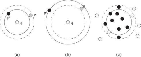
Figure 27.1Examples of (a) an approximate nearest-neighbor p to q with the exact neighbor p*, (b) an approximate farthest-neighbor p to q with the exact neighbor p*, and (c) an approximate range query; here the dark points are reported or counted and the lighter points are not.
To clarify further, a point p is a (1 + ε)-approximate nearest neighbor if its distance is within a constant error factor of the true nearest distance. Although we do not discuss it here, we can extend the definitions to report a sequence of k (1 + ε)-nearest (or (1 − ε)-farthest) neighbors. One may also wonder why the approximate farthest neighbor is defined in absolute terms instead of relative terms as with the nearest version. By observing that the distance from any query point to its farthest neighbor is always at least the radius of the point set OS, one can see that the approximation is as good as the relative approximation. Moreover, if the query point is extremely far from the point set, then a relative approximation could return any point in S, whereas an absolute approximation would require a much more accurate distance.
Although we do not modify our definition here, one can extend this notion and our later theorems to compensate for the problem of query points distant from the point set in nearest-neighbor queries as well. In other words, when the query point is relatively close to the entire data set, we can use the relative error bound, and when it is relatively far away from the entire data set, we can use the absolute error bound.
The approximate range searching problem described above has one-sided false-positive errors. We do not miss any valid points, but we may include erroneous points near the range boundary. It is a simple modification of the query regions to instead get false-negative errors. That is, we could instead require including only points that are inside of Q but allow missing some points that are inside of Q if they are near the border. In fact, for any region Q one could define two epsilon ranges εi and εo for both interior and exterior error bounds and then treat the approximation factor as ε = εi + εo.
There are numerous approaches one may take to solving these problems. Arya et al. [4] introduced a priority search algorithm for visiting nodes in a partition tree to solve nearest-neighbor queries. Using their BBD tree structure, they were able to prove efficient query times. Duncan et al. [10] show how this priority search could also solve farthest-neighbor queries. The nearest and farthest neighbor priority searching algorithms shown in Figures 27.2 and 27.3 come from [8]. In the approximate nearest-neighbor, respectively farthest-neighbor, search, nodes are visited in order of closest node, respectively farthest node. Nodes are extracted via an efficient priority queue, such as the Fibonacci heap [15,16].
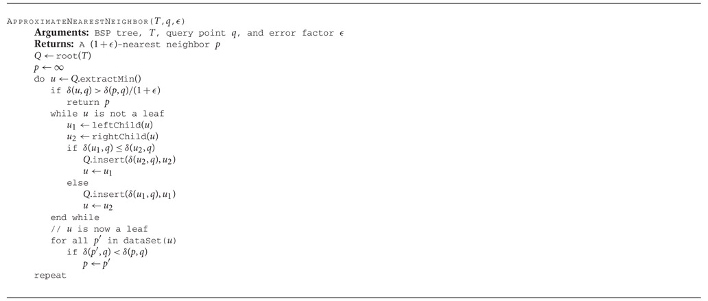
Figure 27.2The basic algorithm to perform nearest-neighbor priority searching.
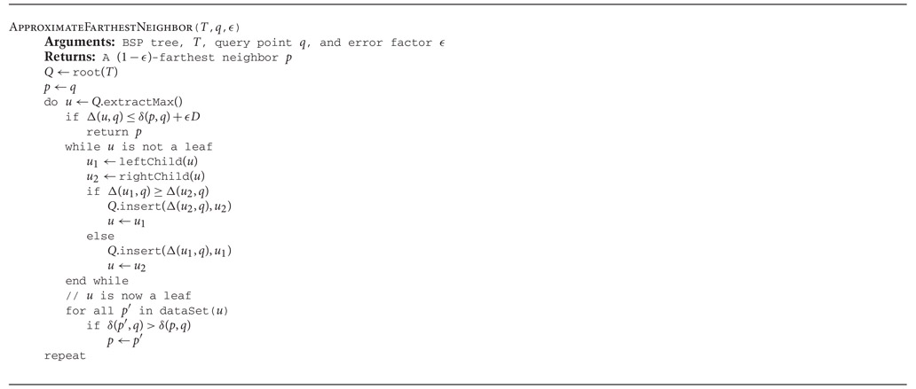
Figure 27.3The basic algorithm to perform farthest-neighbor priority searching.
Introduced by [7], the search technique used for the approximate range query is a modification to the standard range searching algorithm for regular partition trees. We present the algorithm from [8] in Figure 27.4. In this algorithm, we have two different query regions, the inner region Q and the outer region . The goal is to return all points in S that lie inside Q, allowing some points to lie inside Q′ but none outside of Q′. That is Q′ − Q defines a buffer zone that is the only place allowed for erroneous points. Whenever a node u is visited, if u is a leaf node, we simply check all of u’s associated data points. Otherwise, if Ru does not intersect Q, we know that none of its points can lie in Q, and we ignore u and its subtree. If Ru lies completely inside Q′ then all of the data points in its subtree must lie inside Q′, and we report all points. Otherwise, we repeat the process on u’s two child nodes. For an ε-approximate range search, we define Q′ = {p ∈ ℝd|δ(p, Q) ≤ εOQ}. We note that this search algorithm can also be modified to return the count or sum of the weights of the points inside the approximate range rather than explicitly reporting the points.
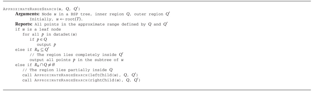
Figure 27.4The basic range search algorithm.
In all of these search algorithms, the essential criteria behind the running time is the observation that a non-terminating node in the search, one that requires expansion of its child nodes, is a node that must cross certain size boundaries. For example, in the approximate range searching algorithm, the only nodes expanded are those whose region lies partially inside Q, else it would be discarded, and partially outside Q′, else it would be completely counted in the output size. A slightly more complex but similar argument applies for nearest and farthest neighbor algorithms. In the next section, we discuss a general theorem providing provable running time bounds for partition trees satisfying a fundamental packing argument.
We are now ready to examine closely a sufficient condition for a data structure to guarantee efficient performance on the aforementioned searches. Before we can proceed, we must first discuss a few more basic definitions presented in Dickerson et al. [12].
Definition 27.3
For any region R, the region annulus with radius r, denoted AR,r is the set of all points p ∈ ℝd such that p ∉ R and δ(p, R) < r. A region R′ pierces an annulus AR,r if and only if there exist two points p, q ∈ R′ such that p ∈ R and q ∉ R ∪ AR,r.
In other words, an annulus AR,r contains all points outside but near the region R. If R were a sphere of radius r′, this would be the standard definition of an annulus with inner radius r′ and outer radius r′ + r. For convenience, when the region and radius of an annulus are understood, we use A. Figure 27.5 illustrates the basic idea of a spherical annulus with multiple piercing regions.
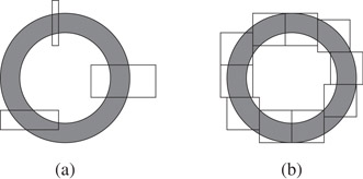
Figure 27.5An example of a simple annulus region (a) with three other regions which pierce this annulus and (b) with several “fat” square regions. Observe that only a limited number of such “fat” squares can pierce the annulus.
The core of the performance analysis for the searches lies in a critical packing argument. The packing lemmas work by bounding the number of disjoint regions that can pierce an annulus and hence simultaneously fit inside the annulus, see Figure 27.5b. When this packing size is small, the searches are efficient. Rather than cover each structure’s search analysis separately, we use the following more generalized notion from Dickerson et al. [12].
Definition 27.4
Given a BSP tree T and a region annulus A, let denote the largest set of disjoint nodes in T whose associated regions pierce A. A class of BSP trees is a ρ(n)-quasi-BAR tree if, for any tree T in the class constructed on a set S of n points in ℝd and any region annulus AR,r, , where VA is the volume of AR,r. The function ρ(n) is called the packing function.
Basically, the packing function ρ(n) represents the maximum number of regions that can pierce any query annulus. By proving that a class of BSP trees is a ρ(n)-quasi-BAR tree, we can automatically inherit the following theorems proven in [4,7,10] and generalized in Reference 12:
Theorem 27.1
Suppose we are given a ρ(n)-quasi-BAR tree T with depth DT = Ω(log n) constructed on a set S of n points in ℝd. For any query point q, the priority search algorithms in Figures 27.2 and 27.3 find respectively a (1 + ε)-nearest and a (1 − ε)-farthest neighbor to q in O(ε1−dρ(n)DT) time.
Theorem 27.2
Suppose we are given a ρ(n)-quasi-BAR tree T with depth DT constructed on a set S of n points in ℝd. For any convex query region Q, the search algorithm in Figure 27.4 solves an ε-approximate range searching query in T in O(ε1−dρ(n)DT) time (plus output size in the reporting case). For any general non-convex query region Q, the time required is O(ε−dρ(n)DT) (plus output size).*
Trivially, ρ(n) is always less than n but this accomplishes little in the means of getting good bounds. Having a class of trees with both a good packing function and low depth helps guarantee good asymptotic performance in answering geometric queries. One approach to finding such classes is to require that all regions produced by the tree be fat. The idea behind this is that there is a limit to the number of disjoint fat regions that pierce an annulus dependent upon the aspect ratio of the regions and the thickness of the annulus. Unfortunately, guaranteeing fat regions and good depth is not readily possible using the standard BSP trees like k-d trees and octrees. Imagine building a k-d tree using only axis-parallel partitioning cuts. Figure 27.6 illustrates such an example. Here the majority of the points are concentrated at a particular corner of a rectangular region. Now, any axis-parallel cut is either too close to the opposing face or does not partition the points in the region well, resulting in large tree depth.
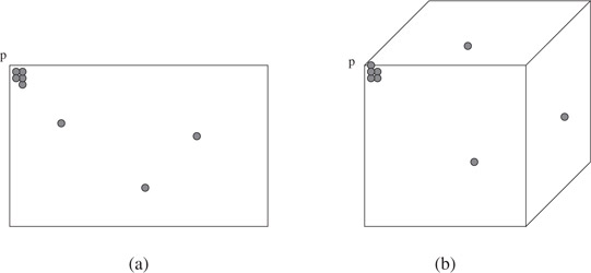
Figure 27.6(a) A bad corner of a simple rectangular region with nearly all of the points clustered near a corner. Notice a cut in either the x or y direction dividing the points located inside p would cause a “skinny” region. (b) The same situation in ℝ3.
Fortunately, there are structures that can provably be shown to be ρ(n)-quasi-BAR trees with small values for ρ(n) and DT. The next few sections discuss some of these structures.
Arya et al. [4] introduced the first BSP tree structure to guarantee both balanced aspect ratio and O(log n) depth. In addition, the aspect ratio achieved allowed them to prove a packing constraint. From this, one can verify that the BBD tree has a packing function of ρ(n) = O(1) where the constant factor depends on the dimension d. In the following section, we describe the basic construction of the BBD tree using terminology from [7].
Every region Ru associated with a node u in a BBD tree is either an outer rectangular box or the set theoretic difference between an outer rectangular box and an inner rectangular box. The size of a box is the length of its longest side and the size of Ru is the size of the outer box. In order to guarantee balanced aspect ratio for these cells, Arya et al. [4] introduced a stickiness restriction on the inner box. Briefly described, an inner box is sticky if the distance between the inner box and every face on the outer box is either 0 or not less than the size of the inner box. Although not necessary to the structure, we shall assume that the aspect ratio of the outer box is no more than two.
The construction of the BBD tree is done by a sequence of alternating splitting and shrinking operations. In the (midpoint) split operation, a region is bisected by a hyperplane cut orthogonal to one of the longest sides. This is essentially the standard type of cut used in a quadtree or octree. Its simplicity, speed of computation, and effectiveness are major reasons for preferring these operations.
The shrink operation partitions a region by a box lying inside the region, creating an inner region. The shrink operation is actually part of a sequence of up to three operations called a centroid shrink. The centroid shrink attempts to partition the region into a small number of subregions Ri such that |Ri| ≤ 2|Ru|/3.
When Ru is simply an outer box, with no inner box, a centroid operation is performed with one shrink operation. The inner partitioning box is found by conceptually applying midpoint split operations recursively on the subregion with the larger number of points. The process stops when the subregion contains no more than 2|Ru|/3 points. The outer box of this subregion is the inner partitioning box for the shrink operation. The other merely conceptual midpoint splits are simply ignored. Choosing this inner box guarantees that both subregions produced by the split have no more than 2|Ru|/3 points. This can be seen by observing that the inner box has no more than 2|Ru|/3 points and also must contain at least |Ru|/3 points. The technique as stated is not theoretically ideal because the number of midpoint split operations computed cannot be bounded. Each midpoint split may not partition even a single point. Arya et al. [4,7] describe a simple solution to this problem, which repeatedly computes the smallest bounding midpoint box using a technique due to Clarkson [17].
When Ru has an inner box associated with it, we cannot simply find another inner box as this would violate the restriction on having only one inner box. Let bi represent the original inner box. The solution is to proceed as in the previous centroid shrink operation, repeatedly applying midpoint split operations on the subregion with the larger number of points. However, we now stop in one of two situations; when the size of the larger subregion either has no more than 2|Ru|/3 points or no longer contains bi. In the former case, let b be the outer box of this subregion. In the latter case, or in the event both cases happen, let b represent the outer box of the subregion prior to this final split. We perform a shrink operation using b as the partitioning box. Since b clearly contains bi, the subregion associated with the original outer box continues to have one inner box, albeit a slightly larger one than its parent. The subregion R1, whose outer box is b, also has one inner box, bi. If |R1| > 2|Ru|/3, we perform a midpoint split on this subregion. Let R2 be the larger subregion formed by this last split, which we know does not contain bi. Since R2 does not contain an inner box, if R2 contains more than 2|Ru|/3 points, we simply perform the basic shrink operation thus dividing R2 into two smaller subregions as well. Clearly, all the subregions produced by this centroid shrink have no more than 2|Ru|/3 points. Figure 27.7 shows the three main operations, splitting, shrinking, and the three-step shrinking process.
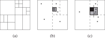
Figure 27.7Examples of (a) multiple iterations of the midpoint split rule, (b) centroid shrinking, with dashed lines representing the conceptual midpoint splits and the highlighted inner box being the actual partition cut, (c) centroid shrinking with an inner box. In the final example, the original inner box is solid, the final midpoint split is shown with slightly extended dotted lines, and the new inner box partition cut is shown shaded in gray.
In addition to this simple version of the BBD tree, there are more flexible variations on this approach. The reader should refer to [4,7] for details on an efficient O(dn log n) construction algorithm and for discussions on some of the BBD variations. To highlight a few options, at any stage in the construction, rather than alternate between shrinking and splitting operations, it is preferable to perform split operations whenever possible, so long as the point set is divided evenly after every few levels, and to use the more costly shrinking operations only when necessary. Another approach is to use a more flexible split operation, a fair split, which attempts to partition the points in the region more evenly. In this case, more care has to be taken to avoid producing skinny regions and to avoid violating the stickiness property; however, as was shown experimentally, the flexibility provides for better experimental performance.
The following theorem summarizes the basic result [4,7]:
Theorem 27.3
Given a set S of n data points in ℝd, in O(dn log n) time it is possible to construct a BBD tree such that
1.The tree has O(n) nodes and depth O(log n),
2.The regions have outer boxes with balanced aspect ratio and inner boxes that are sticky to the outer box,
3.The sizes of the regions are halved after every 2d levels in the tree.
The above conditions imply that the BBD tree is an O(1)-quasi-BAR tree.
The size reduction constraint above helps guarantee a slightly better performance for geometric queries than given for general quasi-BAR trees. In particular, Arya and Mount [7] show that the size reduction allows range queries on BBD trees to be solved in time, or for convex queries plus output size. Duncan [8] later extended the separation of the n and ε dependencies to nearest and farthest neighbor queries showing that the running time for both is O(log n + ε1−d log(1/ε)) for fixed dimension d.
The balanced aspect ratio tree introduced in Reference 9 for the basic two-dimensional case and subsequently revised to higher dimensions in References 8 and 10 can be shown to have a packing function of ρ(n) = O(1) where the constant factor depends on the dimension d and a user-specified aspect ratio parameter α. In the following section, we borrow terminology from [8,10].
Unlike BBD trees, k-d trees, and octrees, BAR trees do not exclusively use axis-orthogonal hyperplane cuts. Instead, to achieve simultaneously the goals of good aspect ratio, balanced depth, and convex regions, cuts in several different directions are used. These directions are called canonical cuts, and the particular choice and size of canonical cuts is essential in creating good BAR trees.
Definition 27.5
The following terms relate to specific cutting directions:
•A canonical cut set, , is a collection of γ not necessarily independent vectors that span ℝd (thus, γ ≥ d).
•A canonical cut direction is any vector .
•A canonical cut is any hyperplane, H, in ℝd with a normal in .
•A canonical region is any region formed by the intersection of a set of hyperspaces defined by canonical cuts, that is, a convex polyhedron in ℝd with every facet having a normal in .
Figure 27.8a shows a region composed of three cut directions (1, 0), (0, 1), and (1, −1), or simply cuts along the x, y, and x − y directions. After cutting the region at the dashed line c, we have two regions R1 and R2. In R2 notice the left side is replaced by the new cut c, and more importantly the diagonal cut is no longer tangential to R2. The following definition describes this property more specifically.
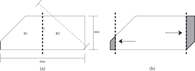
Figure 27.8(a) An example of a canonical region of three cut directions, x,y, and x − y. Observe the three widths highlighted with lines and the min and max widths of the region. The left facet associated with the x direction is drawn in bold. The bold dashed line in the center represents a cut c and the respective subregions R1 and R2. (b) An example of a similar region highlighting the two shield regions associated with the x-direction for α ≈ 4. Notice the size difference between the two shield regions corresponding to the associated facet sizes.
Definition 27.6
A canonical cut c defines a canonical region R, written c ∈ R, if and only if c is tangential to R. In other words, c intersects the border of R. For a canonical region R, any two parallel canonical cuts b, c ∈ R are opposing canonical cuts. For any canonical region R, we define the canonical bounding cuts with respect to a direction to be the two unique opposing canonical cuts normal to and tangent to R. We often refer to these cuts as bi and ci or simply b and c when i is understood from the context. Intuitively, R is “sandwiched” between bi and ci. To avoid confusion, when referring to a canonical cut of a region R, we always mean a canonical bounding cut.
For any canonical bounding cut, c, the facet of c ∈ R, facetc(R), is defined as the region formed by the intersection of R with c.
The canonical set used to define a partition tree can vary from method to method. For example, the standard k-d tree algorithm [18] uses a canonical set composed of all axis-orthogonal directions.
Definition 27.7
For a canonical set and a canonical region R, we define the following terms (see Figure 27.8a):
•For a canonical direction , the width of R in the direction , written widthi(R), is the distance between bi and ci, that is, widthi(R) = δ(bi, ci).
•The maximum side of R is .
•The minimum side of R is .
For simplicity, we also refer to the facets of a region in the same manner. We define the following terms for a facet of a region R, f = facetc(R):
•The width of f in the direction is widthi(f) = δ(bi, ci) where bi and ci are the opposing bounding cuts of f in the direction .
•The maximum side of f is .
•In addition, for any canonical cut c ∈ R, the length of c, lenc(R), is defined as .
When using a canonical cut ci to partition a region R into two pieces R1 and R2 as the cut gets closer to a side of R, one of the two respective regions gets increasingly skinnier. At some point, the region is no longer α-balanced, see Figure 27.8b. This threshold region is referred to as a shield region and is defined in References 8 as the following:
Definition 27.8
Given an α-balanced canonical region R and a canonical cut direction , sweep a cut c′ from the opposing cut bi toward ci. Let P be the region of R between c′ and ci. Sweep c′ until either region P is empty or just before asp(P) > α. If P is not empty, then P has maximum aspect ratio. Call the region P the shield region of ci in R, . Let the maximal outer shield, mosi(R), be the shield region or such that , that is, the maximal outer shield is the shield region with the greater number of points.
Definition 27.9
An α-balanced canonical region, R, is one-cuttable with reduction factor β, where 1/2 ≤ β < 1, if there exists a cut , called a one-cut, dividing R into two subregions R1 and R2 such that the following conditions hold:
1.R1 and R2 are α-balanced canonical regions,
2.|R1| ≤ β|R| and |R2| ≤ β|R|.
Definition 27.10
An α-balanced canonical region, R, is k-cuttable with reduction factor β, for k > 1, if there exists a cut , called a k-cut, dividing R into two subregions R1 and R2 such that the following conditions hold:
1.R1 and R2 are α-balanced canonical regions,
2.|R2| ≤ β|R|,
3.Either |R1| ≤ β|R| or R1 is (k − 1)-cuttable with reduction factor β.
In other words, the sequence of cuts, , results in k + 1 α-balanced canonical regions each containing no more than β|R| points. If the reduction factor β is understood, we simply say R is k-cuttable.
Definition 27.11
For a canonical cut set, , a binary space partition tree T constructed on a set S is a BAR tree with maximum aspect ratio α if every region R ∈ T is α-balanced.
Figure 27.9 illustrates an algorithm to construct a BAR tree from a sequence of k-cuttable regions.

Figure 27.9General BAR tree construction algorithm.
Theorem 27.4
For a canonical cut set, , if every possible α-balanced canonical region is k-cuttable with reduction factor β, then a BAR tree with maximum aspect ratio α can be constructed with depth O(k log1/βn), for any set S of n points in ℝd.
The main challenge in creating a specific instance of a BAR tree is in defining a canonical set such that every possible α-balanced canonical region is k-cuttable with reduction factor β for reasonable choices of α, β, and k. The α-balanced regions produced help BAR trees have the following packing function.
Theorem 27.5
For a canonical cut set, , if every possible α-balanced canonical region is k-cuttable with reduction factor β, then the class of BAR trees with maximum aspect ratio α has a packing function ρ(n) = O(αd) where the hidden constant factor depends on the angles between the various cut directions. For fixed α, this is constant.
Theorems 27.4 and 27.5 immediately show us that approximate geometric nearest-neighbor and farthest-neighbor queries can be solved in O(ε1−d log n) time and approximate geometric range searches for convex and non-convex regions take, respectively, O(ε1−d log n) and O(ε−d log n) plus the output size. As with the BBD tree, in fact, these structures can also be shown to have running times of for nearest-neighbor and farthest-neighbor queries [8] and O(log n + ε1−d) and O(log n + ε−d) for convex and non-convex range queries [7].
Another examination of Figure 27.6 shows why simple axis-orthogonal cuts cannot guarantee k-cuttability. By concentrating a large number of points at an actual corner of the rectangular region, no sequence of axis-orthogonal cuts will divide the points and maintain balanced aspect ratio regions. We can further extend this notion of a bad corner to a general κ-corner associated with a canonical region R.
Definition 27.12
For a canonical cut set and a canonical region R, a κ-corner B ∈ R is a ball with center ρ and radius κ such that, for every cut direction with bounding cuts bi and ci, either bi or ci intersects B, that is, .
When κ = 0, we are not only defining a vertex of a region but a vertex which is tangential to one of every cut direction’s bounding planes. As described in References 8, these corners represent the worst-case placement of points in the region. These corners can always exist in regions. However, if one of the facets associated with this corner has size proportional to (or smaller than) the κ ball, then we can still get close enough to this facet and properly divide the point set without introducing unbalanced regions. The following property formalizes this notion more:
Property 27.13
A canonical cut set satisfies the κ-Corner Property if for any κ ≥ 0 and any canonical region R containing a κ-corner B ∈ R, there exists a canonical cut c ∈ R intersecting B such that for some constant .
In particular, notice that if κ = 0, one of the bounding cutting planes must intersect at a single point. The advantage to this can be seen in the two-dimensional case. Construct any canonical region using any three cutting directions, for simplicity use the two axis-orthogonal cuts and one cut with slope +1. It is impossible to find a κ-corner without having at least one of the three bounding sides be small with respect to the corner. This small side has a matching very small shield region. Unfortunately, having a small shield region does not mean that the initial region is one-cuttable. The points may all still be concentrated within this small shield region. However, it is possible that this small shield region is one-cuttable. In fact, in References 8, it is shown that there exist canonical cut sets that guarantee two-cuttability for sufficient values of α, β, and σ, where the σ parameter is used in the construction. The sufficiency requirements depend only on certain constant properties associated with the angles of the canonical cut set labeled here as and . For specific values of these constants, see Reference 8. Figure 27.10 describes an algorithm to find an appropriate cut.
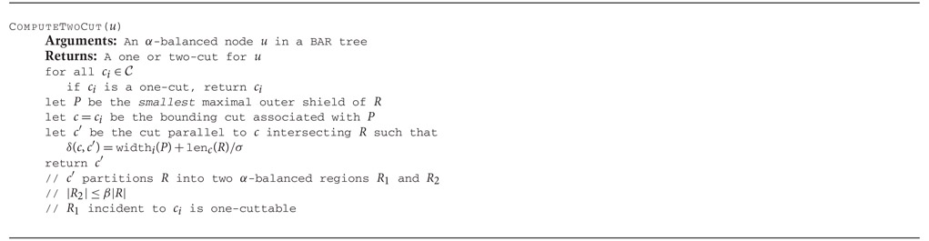
Figure 27.10An algorithm to find either a one or two cut in a region.
The general idea is to find the smallest (in physical size) shield region containing a majority of the points. If none exist, the region must be one-cuttable. Otherwise, we take this shield region and pull the partitioning cut back slightly,* increasing the size of this particular shield region. Given an appropriate cut set and various constant bounds, we can guarantee that this new region is one-cuttable. The following theorems summarize this result [8]:
Theorem 27.6: (Two-Cuttable Theorem)
Suppose we are given a canonical cut set, , which satisfies the κ-Corner Property 27.13. Any α-balanced canonical region R is two-cuttable if the following three conditions are met:
(27.1) |
|---|
(27.2) |
|---|
(27.3) |
|---|
Theorems 27.6 and 27.4 can be combined to yield the following theorem:
Theorem 27.7
Suppose we are given a canonical cut set that satisfies the κ-Corner Property and an . A BAR tree with depth O(d log n) and balancing factor α can be constructed in time, where f and g are constant functions depending on properties of the canonical set. In particular, the running time of the algorithm is O(n log n) for fixed dimensions and fixed canonical sets.
Let us now present two cut sets that do satisfy the κ-Corner Property. The two cut sets we present below are composed of axis-orthogonal cuts and one other set of cuts. Let us give specific names to a few vector directions.
Definition 27.14
A vector v = (x0, x1, x2, …, xd) is
•an axis-orthogonal cut if xi = 0 for all values except one where xj = 1, for example, (0, 0, 1, 0),
•a corner cut if xi = ±1 for all values of i, for example, (1, 1, −1, −1),
•a wedge cut if xi = 0 for all values except two where xj, xi = ±1, for example, (0, 1, −1, 0).
The Corner Cut Canonical Set is the set of all axis-orthogonal cuts and corner cuts. The Wedge Cut Canonical Set is the set of all axis-orthogonal cuts and wedge cuts.
Notice that is Θ(2d) and is Θ(d2). Although the corner cut canonical set does not necessarily have to be as large as this, the complexity of the corner cut itself means sidedness tests take longer than axis-orthogonal and wedge cuts, namely d computations instead of 1 or 2. The above two canonical sets satisfy the κ-Corner Property 27.13 and from Theorem 27.7, we get the following two corollaries [8]:
Corollary 27.1
For the Corner Cut Canonical set , a BAR tree with depth O(d log n) and balancing factor α = Ω(d2) can be constructed in O(n log n) time.
Corollary 27.2
For the Wedge Cut Canonical set , a BAR tree with depth O(d log n) and balancing factor can be constructed in O(n log n) time.
To get the exact values needed, see [8]. However, it is important to note that the α bounds above are overestimates of the minimum value needed. In practice, one should try an initially small value of α, say 6, and when that fails to provide two-cuttability double the value for the lower subtree levels. In this manner, one can arrive at the true minimum value in O(log α) such iterations, if necessary, without having to calculate it. Since the minimum α needed in both cut sets is O(d2), this adds only an O(log (d)) factor to the depth.
One very popular class of BSP tree is the k-d tree, see Chapter 17. Although there are very few theoretical bounds known on these structures, there is a lot of empirical evidence that shows them to be extremely efficient for numerous geometric applications. In particular, one variant the maximum-spread k-d tree has long been considered an ideal k-d tree. Given a set of points S and a particular axis dimension xd, define the spread of S in xd to be the difference between the minimum and maximum coordinates of the points in that dimension. The maximum-spread k-d tree is formed by choosing at each internal node a cutting plane orthogonal to the axis of maximum spread placed at the median point in this direction, see for example [11]. Arya et al. [4] applied the maximum-spread k-d tree to their approximate nearest-neighbor searching algorithm and experimentally showed that they were comparable to the theoretically efficient BBD tree. Later Dickerson et al. [8,12] proved the following theorem regarding maximum-spread k-d trees, referred to there as longest-side k-d trees:
Theorem 27.8
Suppose we are given a maximum-spread k-d tree T constructed on a set S of n points in ℝd. Then the packing function ρ(n) of T for a region annulus A is O(logd−1n). That is, the class of maximum-spread k-d trees is an O(logd−1n)-quasi-BAR tree.
Although the bound is not as good as for BBD trees and BAR trees, the simplicity of the structure yields low constant factors and explains why in practice these trees perform so well. Experimental comparisons to BBD trees and BAR trees verified this result and showed that only for very highly clustered data did the dependency on logd−1n become prominent [4,8]. In practice, unless data is highly clustered and the dimension is moderately large, the maximal-spread k-d tree is an ideal structure to use. However, for such data sets both the BBD tree and the BAR tree revert to the same behavior as the maximal-spread tree, and they perform well even with highly clustered data. Because of its simpler structure, the BBD tree is potentially more practical than the BAR tree.
This work was supported, in part, by the National Science Foundation under grant CCR-0098068.
1.B. Chazelle and E. Welzl. Quasi-optimal range searching in spaces of finite VC-dimension. Discrete Comput. Geom., 4:467–489, 1989.
2.B. Chazelle. Lower bounds on the complexity of polytope range searching. J. Amer. Math. Soc., 2:637–666, 1989.
3.F. P. Preparata and M. I. Shamos. Computational Geometry: An Introduction. Springer-Verlag, New York, NY, 1985.
4.S. Arya, D. M. Mount, N. S. Netanyahu, R. Silverman, A. Wu. An optimal algorithm for approximate nearest neighbor searching in fixed dimensions. J. ACM, 45(6):891–923, 1998.
5.R. A. Finkel, and J. L. Bentley. Quad trees: a data structure for retrieval on composite keys. Acta Inform., 4, pp. 1–9, 1974.
6.P. B. Callahan, and S. R. Kosaraju. A decomposition of multidimensional point sets with applications to k-nearest-neighbors and n-body potential fields. J. ACM, 42:67–90, 1995.
7.S. Arya, and D. M. Mount. Approximate range searching. Comput. Geom., 17(3–4):135–152, 2000.
8.C. A. Duncan. Balanced Aspect Ratio Trees. Ph.D. thesis, Dept. of Computer Science, Johns Hopkins Univ., 1999.
9.C. A. Duncan, M. T. Goodrich, and S. G. Kobourov. Balanced aspect ratio trees and their use for drawing very large graphs. J. Graph Algorithms Appl., 4:19–46, 2000.
10.C. A. Duncan, M. T. Goodrich, and S. G. Kobourov. Balanced aspect ratio trees: Combining the advantages of k-d trees and octrees. J. Algorithms, 38:303–333, 2001.
11.J. H. Friedman, J. L. Bentley, and R. A. Finkel. An algorithm for finding best matches in logarithmic expected time. ACM Trans. Math. Softw., 3:209–226, 1977.
12.M. Dickerson, C. A. Duncan, and M. T. Goodrich. K-D trees are better when cut on the longest side. In ESA: Annual European Symposium on Algorithms, volume 1879 of Lecture Notes Comput. Sci., pages 179–190, 2000.
13.H. Samet. The Design and Analysis of Spatial Data Structures. Addison-Wesley, Reading, MA, 1990.
14.S. Arya and D. M. Mount. Approximate nearest neighbor queries in fixed dimensions. In Proc. 4th ACM-SIAM Sympos. Discrete Algorithms, pages 271–280, 1993.
15.J. R. Driscoll, H. N. Gabow, R. Shrairaman, and R. E. Tarjan. Relaxed heaps: An alternative to Fibonacci heaps with applications to parallel computation. Commun. ACM, 31:1343–1354, 1988.
16.M. Fredman, and R. E. Tarjan. Fibonacci heaps and their uses in improved network optimization problems. J. ACM, 34:596–615, 1987.
17.K. L. Clarkson. Fast algorithms for the all nearest neighbors problem. In Proc. 24th Annu. IEEE Sympos. Found. Comput. Sci., pages 226–232, 1983.
18.J. L. Bentley. Multidimensional binary search trees used for associative searching. Commun. ACM, 18(9):509–517, 1975.
*This chapter has been reprinted from first edition of this Handbook, without any content updates.
*Actually, BBD trees and BAR trees have a slightly better running time for these searches and we mention this in the respective sections.
*This is actually only necessary in dimensions greater than 2.