28. Geometric and Spatial Data Structures in External Memory

Input/Output communication (or simply I/O) between the fast internal memory and the slow external memory (EM, such as disk) can be a bottleneck when processing massive amounts of data, as is the case in many spatial and geometric applications [1]. Problems involving massive amounts of geometric data are ubiquitous in spatial databases, geographic information systems (GIS), constraint logic programming, object-oriented databases, statistics, virtual reality systems, and computer graphics. E-Business and space applications produce petabytes (1015 bytes) of data per year. A major challenge is to develop mechanisms for processing the data, or else much of the data will be useless.

One promising approach for efficient I/O is to design algorithms and data structures that bypass the virtual memory system and explicitly manage their own I/O. We refer to such algorithms and data structures as external memory (or EM) algorithms and data structures. (The terms out-of-core algorithms and I/O algorithms are also sometimes used.)

We concentrate in this chapter on the design and analysis of EM memory data structures for batched and online problems involving geometric and spatial data. Luckily, many problems on geometric objects can be reduced to a small core of problems, such as computing intersections, convex hulls, multidimensional search, range search, stabbing queries, point location, and nearest-neighbor search. In this chapter, we discuss useful paradigms for solving these problems in EM.

28.1.1Disk Model

The three primary measures of performance of an algorithm or data structure are the number of I/O operations performed, the amount of disk space used, and the internal (parallel) computation time. For reasons of brevity, we shall focus in this chapter on only the first two measures. Most of the algorithms we mention run in optimal CPU time, at least for the single processor case.

We can capture the main properties of magnetic disks and multiple disk systems by the commonly used parallel disk model (PDM) (Figure 28.1) introduced by Vitter and Shriver [2]. Data is transferred in large units of blocks of size B so as to amortize the latency of moving the read–write head and waiting for the disk to spin into position. Storage systems such as RAID use multiple disks to get more bandwidth [3,4]. The principal parameters of PDM are the following:

\begin{aligned} N & = problem input data size (in terms of items), \\ M & = size of internal memory (in terms of items), \\ B & = size of disk block (in terms of items), and \\ D & = # independent disks, \end{aligned}

$\begin{aligned} N & = problem input data size (in terms of items), \\ M & = size of internal memory (in terms of items), \\ B & = size of disk block (in terms of items), and \\ D & = # independent disks, \end{aligned}$

where M < N and 1 ≤ DB ≤ M.

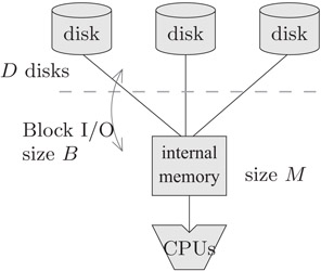
Figure 28.1Parallel disk model.

Queries are naturally associated with online computations, but they can also be done in batched mode. For example, in the batched orthogonal 2-D range searching problem discussed in Section 28.2, we are given a set of N points in the plane and a set of Q queries in the form of rectangles, and the problem is to report the points lying in each of the Q query rectangles. In both the batched and online settings, the number of items reported in response to each query may vary. We thus define two more performance parameters:

\begin{aligned} Q & = number of input queries (for a batched problem) and \\ Z & = query output size (in terms of items) . \end{aligned}

$\begin{aligned} Q & = number of input queries (for a batched problem) and \\ Z & = query output size (in terms of items) . \end{aligned}$

If the problem does not involve queries, we set Q = 0.

It is convenient to refer to some of the above PDM parameters in units of disk blocks rather than in units of data items; the resulting formulas are often simplified. We define the lowercase notation

n = \frac{N}{B}, m = \frac{M}{B}, z = \frac{Z}{B}, q = \frac{Q}{B},

$n = \frac{N}{B}, m = \frac{M}{B}, z = \frac{Z}{B}, q = \frac{Q}{B},$

to be the problem input size, internal memory size, query output size, and number of queries, respectively, in units of disk blocks.

For simplicity, we restrict our attention in this chapter to the single disk case D = 1. The batched algorithms we discuss can generally be sped up by using multiple disks in an optimal manner using the load balancing techniques discussed in Reference 1. Online data structures that use a single disk can generally be transformed automatically by the technique of disk striping to make optimal use of multiple disks [1].

Programs that perform well in terms of PDM will generally perform well when implemented on real systems [1]. More complex and precise models have been formulated [5–7]. Hierarchical (multilevel) memory models are discussed in [1] and its references. Cache-oblivious models are discussed in Chapter 35. Many of the algorithm design techniques we discuss in this chapter, which exploit data locality so as to minimize I/O communication steps, form the basis for algorithms in the other models.

28.1.2Design Criteria for EM Data Structures

The data structures we examine in this chapter are used in batched algorithms and in online settings. In batched problems, no preprocessing is done, and the entire file of data items must be processed, often by streaming the data through the internal memory in one or more passes. Queries are done in a batched manner during the processing. The goal is generally twofold:

•To solve the problem in $O ((n + q) \log_{m} n + z)$ $O ((n + q) \log_{m} n + z)$ I/Os

•To use only a linear number O(n + q) of blocks of disk storage

Most nontrivial problems require the same number of I/Os as does sorting. In particular, criterion B1 is related to the I/O complexity of sorting N items in the PDM model, which is O(n log_m n) [1].

Online data structures support query operations in a continuous manner. When the data items do not change and the data structure can be preprocessed before any queries are made, the data structure is known as static. When the data structure supports insertions and deletions of items, intermixed with the queries, the data structure is called dynamic. The primary theoretical challenges in the design and analysis of online EM data structures are threefold:

•To answer queries in O(log_B N + z) I/Os

•To use only a linear number O(n) of blocks of disk storage

•To do updates (in the case of dynamic data structures) in O(log_B N) I/Os

Criteria O1–O3 correspond to the natural lower bounds for online search in the comparison model. The three criteria are problem dependent, and for some problems they cannot be met. For dictionary queries, we can do better using hashing, achieving O(1) I/Os per query on the average.

Criterion O1 combines together the O(log_B N) I/O cost for the search with the O(⌈z⌉) I/O cost for reporting the output. When one cost is much larger than the other, the query algorithm has the extra freedom to follow a filtering paradigm [8], in which both the search component and the output reporting are allowed to use the larger number of I/Os. For example, when the output size Z is large, the search component can afford to be somewhat sloppy as long as it doesn’t use more than O(z) I/Os; when Z is small, the Z output items do not have to reside compactly in only O(⌈z⌉) blocks. Filtering is an important design paradigm in online EM data structures.

For many of the batched and online problems we consider, there is a data structure (such as a scanline structure or binary search tree) for the internal memory version of the problem that can answer each query in O(log N + Z) CPU time, but if we use the same data structure naively in an EM setting (using virtual memory to handle page management), a query may require Ω(log N + Z) I/Os, which is excessive.^*

The goal for online algorithms is to build locality directly into the data structure and explicitly manage I/O so that the log N and Z terms in the I/O bounds of the naive approach are replaced by log_B N and z, respectively. The relative speedup in I/O performance, namely (log N + Z)/(log_B N + z), is at least (log N)/ log_B N = log B, which is significant in practice, and it can be as much as Z/z = B for large Z.

For batched problems, the I/O performance can be improved further, since the answers to the queries do not need to be provided immediately but can be reported as a group at the end of the computation. For the batched problems we consider in this chapter, the Q = qB queries collectively use O(q log_m n + z) I/Os, which is about B times less than a naive approach.

28.1.3Overview of Chapter

In the next section, we discuss batched versions of geometric search problems. One of the primary methods used for batched geometric problems is distribution sweeping, which uses a data structure reminiscent of the distribution paradigm in external sorting. Other useful batched techniques include persistent B-trees, batched filtering, external fractional cascading, external marriage-before-conquest, and batched incremental construction.

The most popular EM online data structure is the B-tree structure, which provides excellent performance for dictionary operations and one-dimensional range searching. We give several variants and applications of B-trees in Section 28.3. We look at several aspects of multidimensional range search in Section 28.4 and related problems such as stabbing queries and point location. Data structures for other variants and related problems such as nearest-neighbor search are discussed in Section 28.5. Dynamic and kinetic data structures are discussed in Section 28.6. The content of this chapter comes largely from portions of a survey article by Vitter [9]. A more comprehensive manuscript on EM data structures appears in Reference 1.

28.2EM Algorithms for Batched Geometric Problems

Advances in recent years have allowed us to solve a variety of batched geometric problems optimally, meeting both optimality Criteria B1 and B2 of Section 28.1.2. These problems include

1.Computing the pairwise intersections of N segments in the plane and their trapezoidal decomposition

2.Finding all intersections between N nonintersecting red line segments and N nonintersecting blue line segments in the plane

3.Answering Q orthogonal 2-D range queries on N points in the plane (i.e., finding all the points within the Q query rectangles)

4.Constructing the 2-D and 3-D convex hull of N points

5.Voronoi diagram and Triangulation of N points in the plane

6.Performing Q point location queries in a planar subdivision of size N

7.Finding all nearest neighbors for a set of N points in the plane

8.Finding the pairwise intersections of N orthogonal rectangles in the plane

9.Computing the measure of the union of N orthogonal rectangles in the plane

10.Computing the visibility of N segments in the plane from a point

11.Performing Q ray-shooting queries in 2-D Constructive Solid Geometry (CSG) models of size N

Goodrich et al. [10], Zhu [11], Arge et al. [12,13], and Crauser et al. [14,15] developed EM algorithms for those problems using these EM paradigms for batched problems:

Distribution sweeping, a generalization of the sorting distribution paradigm [1] for “externalizing” plane sweep algorithms.

Persistent B-trees: An oﬄine method for constructing an optimal space persistent version of the B-tree data structure (see Section 28.3.1), yielding a factor of B improvement over the generic persistence techniques of Driscoll et al. [16].

Batched filtering: A general method for performing simultaneous EM searches in data structures that can be modeled as planar layered directed acyclic graphs; it is useful for 3-D convex hulls and batched point location. Multisearch on parallel computers is considered in Reference 17.

External fractional cascading: An EM analogue to fractional cascading on a segment tree, in which the degree of the segment tree is O(m^α) for some constant 0 < α ≤ 1. Batched queries can be performed efficiently using batched filtering; online queries can be supported efficiently by adapting the parallel algorithms of work of Tamassia and Vitter [18] to the I/O setting.

External marriage-before-conquest: An EM analogue to the technique of Kirkpatrick and Seidel [19] for performing output-sensitive convex hull constructions.

Batched incremental construction: A localized version of the randomized incremental construction paradigm of Clarkson and Shor [20], in which the updates to a simple dynamic data structure are done in a random order, with the goal of fast overall performance on the average. The data structure itself may have bad worst-case performance, but the randomization of the update order makes worst-case behavior unlikely. The key for the EM version so as to gain the factor of B I/O speedup is to batch together the incremental modifications.

For illustrative purposes, we focus in the remainder of this section primarily on the distribution sweep paradigm [10], which is a combination of the distribution paradigm for sorting [1] and the well-known sweeping paradigm from computational geometry [21,22]. As an example, let us consider how to achieve optimality Criteria B1 and B2 for computing the pairwise intersections of N orthogonal segments in the plane, making use of the following recursive distribution sweep. At each level of recursion, the region under consideration is partitioned into Θ(m) vertical slabs, each containing Θ(N/m) of the segments’ endpoints.

We sweep a horizontal line from top to bottom to process the N segments. When the sweep line encounters a vertical segment, we insert the segment into the appropriate slab. When the sweep line encounters a horizontal segment h, as pictured in Figure 28.2, we report h’s intersections with all the “active” vertical segments in the slabs that are spanned completely by h. (A vertical segment is “active” if it intersects the current sweep line; vertical segments that are found to be no longer active are deleted from the slabs.) The remaining two end portions of h (which “stick out” past a slab boundary) are passed recursively to the next level, along with the vertical segments. The downward sweep then proceeds. After the initial sorting (to get the segments with respect to the y-dimension), the sweep at each of the O(log_m n) levels of recursion requires O(n) I/Os, yielding the desired bound in B1 of $O ((n + q) \log_{m} n + z)$ $O ((n + q) \log_{m} n + z)$ . Some timing experiments on distribution sweeping appear in Reference 23. Arge et al. [13] develop a unified approach to distribution sweep in higher dimensions.

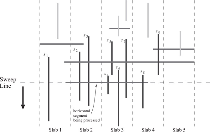
Figure 28.2Distribution sweep used for finding intersections among N orthogonal segments. The vertical segments currently stored in the slabs are indicated in bold (namely, s1, s2, …, s9). Segments s5 and s9 are not active but have not yet been deleted from the slabs. The sweep line has just advanced to a new horizontal segment that completely spans slabs 2 and 3, so slabs 2 and 3 are scanned and all the active vertical segments in slabs 2 and 3 (namely, s2, s3, s4, s6, s7) are reported as intersecting the horizontal segment. In the process of scanning slab 3, segment s5 is discovered to be no longer active and can be deleted from slab 3. The end portions of the horizontal segment that “stick out” into slabs 1 and 4 are handled by the lower levels of recursion, where the intersection with s8 is eventually discovered.

A central operation in spatial databases is spatial join. A common preprocessing step is to find the pairwise intersections of the bounding boxes of the objects involved in the spatial join. The problem of intersecting orthogonal rectangles can be solved by combining the previous sweep line algorithm for orthogonal segments with one for range searching. Arge et al. [13] take a more unified approach using distribution sweep, which is extendible to higher dimensions. The active objects that are stored in the data structure in this case are rectangles, not vertical segments. The authors choose the branching factor to be $Θ (\sqrt{m})$ $Θ (\sqrt{m})$ . Each rectangle is associated with the largest contiguous range of vertical slabs that it spans. Each of the possible contiguous ranges of slabs is called a multislab. The reason why the authors choose the branching factor to be $Θ (\sqrt{m})$ $Θ (\sqrt{m})$ rather than Θ(m) is so that the number of multislabs is Θ(m), and thus there is room in internal memory for a buffer for each multislab. The height of the tree remains O(log_m n).

The algorithm proceeds by sweeping a horizontal line from top to bottom to process the N rectangles. When the sweep line first encounters a rectangle R, we consider the multislab lists for all the multislabs that R intersects. We report all the active rectangles in those multislab lists, since they are guaranteed to intersect R. (Rectangles no longer active are discarded from the lists.) We then extract the left and right end portions of R that partially “stick out” past slab boundaries, and we pass them down to process in the next lower level of recursion. We insert the remaining portion of R, which spans complete slabs, into the list for the appropriate multislab. The downward sweep then continues. After the initial sorting preprocessing, each of the O(log_m n) sweeps (one per level of recursion) takes O(n) I/Os, yielding the desired bound $O ((n + q) \log_{m} n + z)$ $O ((n + q) \log_{m} n + z)$ .

The resulting algorithm, called Scalable Sweeping-Based Spatial Join (SSSJ) [13,24], outperforms other techniques for rectangle intersection. It was tested against two other sweep line algorithms: the Partition-Based Spatial Merge (QPBSM) used in Paradise [25] and a faster version called MPBSM that uses an improved dynamic data structure for intervals [24]. The TPIE (Transparent Parallel I/O Environment) system [26–28] served as the common implementation platform. The algorithms were tested on several data sets. The timing results for the two data sets in Figure 28.3a and b are given in Figure 28.3c and d, respectively. The first data set is the worst case for sweep line algorithms; a large fraction of the line segments in the file are active (i.e., they intersect the current sweep line). The second data set is a best case for sweep line algorithms, but the two PBSM algorithms have the disadvantage of making extra copies of the rectangles. In both cases, SSSJ shows considerable improvement over the PBSM-based methods. In other experiments done on more typical data, such as TIGER/line road data sets [29], SSSJ and MPBSM perform about 30% faster than does QPBSM. The conclusion we draw is that SSSJ is as fast as other known methods on typical data, but unlike other methods, it scales well even for worst-case data. If the rectangles are already stored in an index structure, such as the R-tree index structure we consider in Section 28.4.2, hybrid methods that combine distribution sweep with inorder traversal often perform best [30].

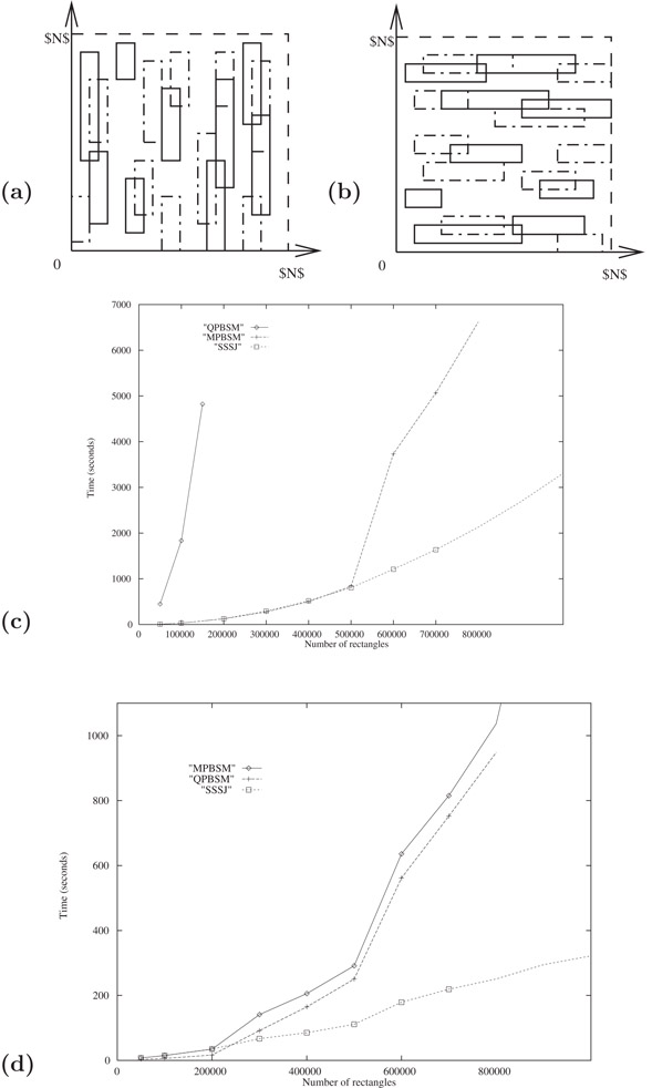
Figure 28.3Comparison of SSSJ with the original PBSM (QPBSM) and a new variant (MPBSM). Each data set contains N/2 red rectangles (designated by solid sides) and N/2 blue rectangles (designated by dashed sides), and the goal is to find all intersections between red rectangles and blue rectangles. In each data set shown, the number of intersections is O(N): (a) data set 1 consists of tall, skinny (vertically aligned) rectangles; (b) data set 2 consists of short, wide (horizontally aligned) rectangles; (c) running times on data set 1; and (d) running times on data set 2.

For the problem of finding all intersections among N line segments, Arge et al. [12] give an efficient algorithm based upon distribution sort, but the output component of the I/O bound is slightly nonoptimal: z log_m n rather than z. Crauser et al. [14,15] attain the optimal I/O bound of criterion B1, namely $O ((n + q) \log_{m} n + z)$ $O ((n + q) \log_{m} n + z)$ , by constructing the trapezoidal decomposition for the intersecting segments using an incremental randomized construction. For I/O efficiency, they do the incremental updates in a series of batches, in which the batch size is geometrically increasing by a factor of m.

Online issues also arise in the analysis of batched EM algorithms. In practice, batched algorithms must adapt in a robust and online way when the memory allocation changes, and online techniques can play an important role. Some initial work has been done on memory-adaptive EM algorithms in a competitive framework [31].

28.3EM Tree Data Structures

In this section, we consider the basic online EM data structures for storing and querying spatial data in one dimension. The dictionary problem is an important special case, which can be solved efficiently in the average case by use of hashing. However, hashing does not support sequential search in a natural way, such as retrieving all the items with key value in a specified range. Some clever work has been done on order-preserving hash functions, in which items with sequential keys are stored in the same block or in adjacent blocks, but the search performance is less robust and tends to deteriorate because of unwanted collisions (see References 1 and 32 for surveys).

A more effective EM approach for geometric queries is to use multiway trees, which we explore in this section. For illustration, we use orthogonal range search as our canonical problem. It is a fundamental database primitive in spatial databases and GIS, and it includes dictionary lookup as a special case. A range query, for a given d-dimensional rectangle, returns all the points in the interior of the rectangle. Other types of spatial queries include point location queries, ray shooting queries, nearest-neighbor queries, and intersection queries, but for brevity we restrict our attention primarily to range searching.

Spatial data structures tend to be of two types: space-driven or data-driven. Quad trees and grid files are space-driven since they are based upon a partitioning of the embedding space, somewhat akin to using order-preserving hash functions, whereas methods like R-trees and kd-trees are organized by partitioning the data items themselves. We shall discuss primarily the latter type in this chapter.

28.3.1B-trees and Variants

Tree-based data structures arise naturally in the online setting, in which the data can be updated and queries must be processed immediately. Binary trees have a host of applications in the (internal memory) RAM model. In order to exploit block transfer, trees in EM generally use a block for each node, which can store Θ(B) pointers and data values.

The well-known balanced multiway B-tree due to Bayer and McCreight [33–35] is the most widely used nontrivial EM data structure. The degree of each node in the B-tree (with the exception of the root) is required to be Θ(B), which guarantees that the height of a B-tree storing N items is roughly log_B N. B-trees support dynamic dictionary operations and one-dimensional range search optimally in linear space, O(log_B N) I/Os per insert or delete, and O(log_B N + z) I/Os per query, where Z = zB is the number of items output. When a node overflows during an insertion, it splits into two half-full nodes, and if the splitting causes the parent node to overflow, the parent node splits, and so on. Splittings can thus propagate up to the root, which is how the tree grows in height. Deletions are handled in a symmetric way by merging nodes.

In the B⁺-tree variant, pictured in Figure 28.4, all the items are stored in the leaves, and the leaves are linked together in symmetric order to facilitate range queries and sequential access.

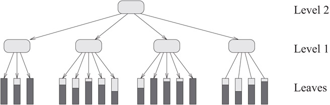
Figure 28.4B⁺-tree multiway search tree. Each internal and leaf node corresponds to a disk block. All the items are stored in the leaves; the darker portion of each leaf block indicates its relative fullness. The internal nodes store only key values and pointers, Θ(B) of them per node. Although not indicated here, the leaf blocks are linked sequentially.

The internal nodes store only key values and pointers and thus can have a higher branching factor. In the most popular variant of B⁺-trees, called B*-trees, splitting can usually be postponed when a node overflows by “sharing” the node’s data with one of its adjacent siblings. The node needs to be split only if the sibling is also full; when that happens, the node splits into two, and its data and those of its full sibling are evenly redistributed, making each of the three nodes about two-thirds full. This local optimization reduces the number of times new nodes must be created and thus increases the storage utilization. And since there are fewer nodes in the tree, search I/O costs are lower. When no sharing is done (as in B⁺-trees), Yao [36] shows that nodes are roughly ln2 ≈ 69% full on the average, assuming random insertions. With sharing (as in B*-trees), the average storage utilization increases to about 2ln(3/2) ≈ 81% [37,38]. Storage utilization can be increased further by sharing among several siblings, at the cost of more complicated insertions and deletions. Some helpful space-saving techniques borrowed from hashing are partial expansions [39] and use of overflow nodes [40].

A cross between B-trees and hashing, where each subtree rooted at a certain level of the B-tree is instead organized as an external hash table, was developed by Litwin and Lomet [41] and further studied in References 42 and 43. O’Neil [44] proposed a B-tree variant called the SB-tree that clusters together on the disk symmetrically ordered nodes from the same level so as to optimize range queries and sequential access. Rao and Ross [45,46] use similar ideas to exploit locality and optimize search tree performance in internal memory. Reducing the number of pointers allows a higher branching factor and thus faster search.

Partially persistent versions of B-trees have been developed by Becker et al. [47] and Varman and Verma [48]. By persistent data structure, we mean that searches can be done with respect to any timestamp y [16,49]. In a partially persistent data structure, only the most recent version of the data structure can be updated. In a fully persistent data structure, any update done with timestamp y affects all future queries for any time after y. An interesting open problem is whether B-trees can be made fully persistent. Salzberg and Tsotras [50] survey work done on persistent access methods and other techniques for time-evolving data. Lehman and Yao [51], Mohan [52], and Lomet and Salzberg [53] explore mechanisms to add concurrency and recovery to B-trees. Other variants are discussed in Chapter 16.

28.3.2Weight-Balanced B-trees

Arge and Vitter [54] introduce a powerful variant of B-trees called weight-balanced B-trees, with the property that the weight of any subtree at level h (i.e., the number of nodes in the subtree rooted at a node of height h) is Θ(ah), for some fixed parameter a of order B. By contrast, the sizes of subtrees at level h in a regular B-tree can differ by a multiplicative factor that is exponential in h. When a node on level h of a weight-balanced B-tree gets rebalanced, no further rebalancing is needed until its subtree is updated Ω(ah) times. Weight-balanced B-trees support a wide array of applications in which the I/O cost to rebalance a node of weight w is O(w); the rebalancings can be scheduled in an amortized (and often worst-case) way with only O(1) I/Os. Such applications are very common when the nodes have secondary structures, as in multidimensional search trees, or when rebuilding is expensive. Agarwal et al. [55] apply weight-balanced B-trees to convert partition trees such as kd-trees, BBD trees, and BAR trees, which were designed for internal memory, into efficient EM data structures.

Weight-balanced trees called BB[α]-trees [56,57] have been designed for internal memory; they maintain balance via rotations, which is appropriate for binary trees, but not for the multiway trees needed for EM. In contrast, weight-balanced B-trees maintain balance via splits and merges.

Weight-balanced B-trees were originally conceived as part of an optimal dynamic EM interval tree structure for stabbing queries and a related EM segment tree structure. We discuss their use for stabbing queries and other types of range queries in Sections 28.4.3 through 28.4.5. They also have applications in the (internal memory) RAM model [54,58], where they offer a simpler alternative to BB[α]-trees. For example, by setting a to a constant in the EM interval tree based upon weight-balanced B-trees, we get a simple worst-case implementation of interval trees [59,60] in internal memory. Weight-balanced B-trees are also preferable to BB[α]-trees for purposes of augmenting one-dimensional data structures with range restriction capabilities [61].

28.3.3Parent Pointers and Level-Balanced B-trees

It is sometimes useful to augment B-trees with parent pointers. For example, if we represent a total order via the leaves in a B-tree, we can answer order queries such as “Is x < y in the total order?” by walking upwards in the B-tree from the leaves for x and y until we reach their common ancestor. Order queries arise in online algorithms for planar point location and for determining reachability in monotone subdivisions [62]. If we augment a conventional B-tree with parent pointers, then each split operation costs Θ(B) I/Os to update parent pointers, although the I/O cost is only O(1) when amortized over the updates to the node. However, this amortized bound does not apply if the B-tree needs to support cut and concatenate operations, in which case the B-tree is cut into contiguous pieces and the pieces are rearranged arbitrarily. For example, reachability queries in a monotone subdivision are processed by maintaining two total orders, called the leftist and rightist orders, each of which is represented by a B-tree. When an edge is inserted or deleted, the tree representing each order is cut into four consecutive pieces, and the four pieces are rearranged via concatenate operations into a new total order. Doing cuts and concatenation via conventional B-trees augmented with parent pointers will require Θ(B) I/Os per level in the worst case. Node splits can occur with each operation (unlike the case where there are only inserts and deletes), and thus there is no convenient amortization argument that can be applied.

Agarwal et al. [62] describe an interesting variant of B-trees called level-balanced B-trees for handling parent pointers and operations such as cut and concatenate. The balancing condition is “global.” The data structure represents a forest of B-trees in which the number of nodes on level h in the forest is allowed to be at most N_h = 2N/(b/3)h, where b is some fixed parameter in the range 4 < b < B/2. It immediately follows that the total height of the forest is roughly log_b N.

Unlike previous variants of B-trees, the degrees of individual nodes of level-balanced B-trees can be arbitrarily small, and for storage purposes, nodes are packed together into disk blocks. Each node in the forest is stored as a node record (which points to the parent’s node record) and a doubly linked list of child records (which point to the node records of the children). There are also pointers between the node record and the list of child records. Every disk block stores only node records or only child records, but all the child records for a given node must be stored in the same block (possibly with child records for other nodes). The advantage of this extra level of indirection is that cuts and concatenates can usually be done in only O(1) I/Os per level of the forest. For example, during a cut, a node record gets split into two, and its list of child nodes is chopped into two separate lists. The parent node must therefore get a new child record to point to the new node. These updates require O(1) I/Os except when there is not enough space in the disk block of the parent’s child records, in which case the block must be split into two, and extra I/Os are needed to update the pointers to the moved child records. The amortized I/O cost, however, is only O(1) per level, since each update creates at most one node record and child record at each level. The other dynamic update operations can be handled similarly.

All that remains is to reestablish the global level invariant when a level gets too many nodes as a result of an update. If level h is the lowest such level out of balance, then level h and all the levels above it are reconstructed via a postorder traversal in O(N_h) I/Os so that the new nodes get degree Θ(b) and the invariant is restored. The final trick is to construct the new parent pointers that point from the Θ(N_{h − 1}) = Θ(bN_h) node records on level h − 1 to the Θ(N_h) level-h nodes. The parent pointers can be accessed in a blocked manner with respect to the new ordering of the nodes on level h. By sorting, the pointers can be rearranged to correspond to the ordering of the nodes on level h − 1, after which the parent pointer values can be written via a linear scan. The resulting I/O cost is , which can be amortized against the Θ(N_h) updates that occurred since the last time the level-h invariant was violated, yielding an amortized update cost of I/Os per level.

Order queries such as “Does leaf x precede leaf y in the total order represented by the tree?” can be answered using O(log_B N) I/Os by following parent pointers starting at x and y. The update operations insert, delete, cut, and concatenate can be done in I/Os amortized, for any 2 ≤ b ≤ B/2, which is never worse than by appropriate choice of b.

Using the multislab decomposition we discuss in Section 28.4.3, Agarwal et al. [62] apply level-balanced B-trees in a data structure for point location in monotone subdivisions, which supports queries and (amortized) updates in I/Os. They also use it to dynamically maintain planar st-graphs using I/Os (amortized) per update, so that reachability queries can be answered in O(log_B N) I/Os (worst-case). (Planar st-graphs are planar directed acyclic graphs with a single source and a single sink.) An interesting open question is whether level-balanced B-trees can be implemented in O(log_B N) I/Os per update. Such an improvement would immediately give an optimal dynamic structure for reachability queries in planar st-graphs.

28.3.4Buffer Trees

An important paradigm for constructing algorithms for batched problems in an internal memory setting is to use a dynamic data structure to process a sequence of updates. For example, we can sort N items by inserting them one by one into a priority queue, followed by a sequence of N delete_min operations. Similarly, many batched problems in computational geometry can be solved by dynamic plane sweep techniques. For example, in Section 28.2 we showed how to compute orthogonal segment intersections by dynamically keeping track of the active vertical segments (i.e., those hit by the horizontal sweep line); we mentioned a similar algorithm for orthogonal rectangle intersections.

However, if we use this paradigm naively in an EM setting, with a B-tree as the dynamic data structure, the resulting I/O performance will be highly nonoptimal. For example, if we use a B-tree as the priority queue in sorting or to store the active vertical segments hit by the sweep line, each update and query operation will take O(log_B N) I/Os, resulting in a total of O(N log_B N) I/Os, which is larger than the optimal bound O(n log_m n) by a substantial factor of roughly B. One solution suggested in Reference 63 is to use a binary tree data structure in which items are pushed lazily down the tree in blocks of B items at a time. The binary nature of the tree results in a data structure of height O(log n), yielding a total I/O bound of O(n log n), which is still nonoptimal by a significant log m factor.

Arge [64] developed the elegant buffer tree data structure to support batched dynamic operations, as in the sweep line example, where the queries do not have to be answered right away or in any particular order. The buffer tree is a balanced multiway tree, but with degree Θ(m) rather than degree Θ(B), except possibly for the root. Its key distinguishing feature is that each node has a buffer that can store Θ(M) items (i.e., Θ(m) blocks of items). Items in a node are pushed down to the children when the buffer fills. Emptying a full buffer requires Θ(m) I/Os, which amortizes the cost of distributing the M items to the Θ(m) children. Each item thus incurs an amortized cost of O(m/M) = O(1/B) I/Os per level, and the resulting cost for queries and updates is I/Os amortized.

Buffer trees have an ever-expanding list of applications. They can be used as a subroutine in the standard sweep line algorithm in order to get an optimal EM algorithm for orthogonal segment intersection. Arge showed how to extend buffer trees to implement segment trees [65] in EM in a batched dynamic setting by reducing the node degrees to $Θ (\sqrt{m})$ $Θ (\sqrt{m})$ and by introducing multislabs in each node, which were explained in Section 28.2 for the related batched problem of intersecting rectangles. Buffer trees provide a natural amortized implementation of priority queues for time-forward processing applications such as discrete event simulation, sweeping, and list ranking [66]. Govindarajan et al. [67] use time-forward processing to construct a well-separated pair decomposition of N points in d dimensions in $O (n \log_{m} n)$ $O (n \log_{m} n)$ I/Os, and they apply it to the problems of finding the K nearest neighbors for each point and the K closest pairs. Brodal and Katajainen [68] provide a worst-case optimal priority queue, in the sense that every sequence of B insert and delete_min operations requires only O(log_m n) I/Os. Practical implementations of priority queues based upon these ideas are examined in References 69 and 70. In Section 28.4.2, we report on some timing experiments involving buffer trees for use in bulk loading of R-trees. Further experiments on buffer trees appear in Reference 71.

28.4Spatial Data Structures and Range Search

In this section, we consider online EM data structures for storing and querying spatial data. A fundamental database primitive in spatial databases and GIS is range search, which includes dictionary lookup as a special case. An orthogonal range query, for a given d-dimensional rectangle, returns all the points in the interior of the rectangle. In this section, we use range searching (especially for the orthogonal 2-D case when d = 2) as the canonical query operation on spatial data. Other types of spatial queries include point location, ray shooting, nearest neighbor, and intersection queries, but for brevity we restrict our attention primarily to range searching.

There are two types of spatial data structures: data-driven and space-driven. R-trees and kd-trees are data-driven since they are based upon a partitioning of the data items themselves, whereas space-driven methods such as quad trees and grid files are organized by a partitioning of the embedding space, akin to order-preserving hash functions. In this section, we discuss primarily data-driven data structures.

Multidimensional range search is a fundamental primitive in several online geometric applications, and it provides indexing support for constraint and object-oriented data models (see Reference 72 for background). We have already discussed multidimensional range searching in a batched setting in Section 28.2. In this section, we concentrate on data structures for the online case.

For many types of range searching problems, it is very difficult to develop theoretically optimal algorithms and data structures. Many open problems remain. The goal for online data structures is typically to achieve the three optimality Criteria O1–O3 of Section 28.1.2.

We explain in Section 28.4.6 that under a fairly general computational model for general 2-D orthogonal queries, as pictured in Figure 28.5d, it is impossible to satisfy Criteria O1 and O2 simultaneously. At least blocks of disk space must be used to achieve a query bound of I/Os per query, for any constant c [73]. Three natural questions arise:

•What sort of performance can be achieved when using only a linear amount of disk space? In Sections 28.4.1 and 28.4.2, we discuss some of the linear-space data structures used extensively in practice. None of them come close to satisfying Criteria O1 and O3 for range search in the worst case, but in typical case scenarios they often perform well. We devote Section 28.4.2 to R-trees and their variants, which are the most popular general-purpose spatial structures developed to date.

•Since the lower bound applies only to general 2-D rectangular queries, are there any data structures that meet Criteria O1–O3 for the important special cases of 2-D range searching pictured in Figure 28.5a–c? Fortunately the answer is yes. We show in Sections 28.4.3 and 28.4.4 how to use a “bootstrapping” paradigm to achieve optimal search and update performance.

•Can we meet Criteria O1 and O2 for general four-sided range searching if the disk space allowance is increased to blocks? Yes again! In Section 28.4.5, we show how to adapt the optimal structure for three-sided searching in order to handle general four-sided searching in optimal search cost. The update cost, however, is not known to be optimal.

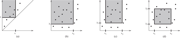
Figure 28.5Different types of 2-D orthogonal range queries: (a) diagonal corner two-sided 2-D query (equivalent to a stabbing query, cf. Section 28.4.3), (b) two-sided 2-D query, (c) three-sided 2-D query, and (d) general four-sided 2-D query.

In Section 28.5, we discuss other scenarios of range search dealing with three dimensions and nonorthogonal queries. We discuss the lower bounds for 2-D range searching in Section 28.4.6.

28.4.1Linear-Space Spatial Structures

Grossi and Italiano [74] construct an elegant multidimensional version of the B-tree called the cross tree. Using linear space, it combines the data-driven partitioning of weight-balanced B-trees (cf. Section 28.3.2) at the upper levels of the tree with the space-driven partitioning of methods such as quad trees at the lower levels of the tree. For d > 1, d-dimensional orthogonal range queries can be done in O(n^{1 − 1/d} + z) I/Os, and inserts and deletes take O(log_B N) I/Os. The O-tree of Kanth and Singh [75] provides similar bounds. Cross trees also support the dynamic operations of cut and concatenate in O(n^{1 − 1/d}) I/Os. In some restricted models for linear-space data structures, the 2-D range search query performance of cross trees and O-trees can be considered to be optimal, although it is much larger than the logarithmic bound of Criterion O1.

One way to get multidimensional EM data structures is to augment known internal memory structures, such as quad trees and kd-trees, with block-access capabilities. Examples include kd–B-trees [76], buddy trees [77], and hB-trees [78,79]. Grid files [80–82] are a flattened data structure for storing the cells of a two-dimensional grid in disk blocks. Another technique is to “linearize” the multidimensional space by imposing a total ordering on it (a so-called space-filling curve), and then the total order is used to organize the points into a B-tree [83–85]. Linearization can also be used to represent nonpoint data, in which the data items are partitioned into one or more multidimensional rectangular regions [86,87]. All the methods described in this paragraph use linear space, and they work well in certain situations; however, their worst-case range query performance is no better than that of cross trees, and for some methods, such as grid files, queries can require Θ(n) I/Os, even if there are no points satisfying the query. We refer the reader to References 32, 88, and 89 for a broad survey of these and other interesting methods. Space-filling curves arise again in connection with R-trees, which we describe next.

28.4.2R-trees

The R-tree of Guttman [90] and its many variants are a practical multidimensional generalization of the B-tree for storing a variety of geometric objects, such as points, segments, polygons, and polyhedra, using linear disk space. Internal nodes have degree Θ(B) (except possibly the root), and leaves store Θ(B) items. Each node in the tree has associated with it a bounding box (or bounding polygon) of all the items in its subtree. A big difference between R-trees and B-trees is that in R-trees the bounding boxes of sibling nodes are allowed to overlap. If an R-tree is being used for point location, for example, a point may lie within the bounding box of several children of the current node in the search. In that case the search must proceed to all such children.

In the dynamic setting, there are several popular heuristics for where to insert new items into an R-tree and how to rebalance it (see Chapter 22 and References 32, 88, and 91 for a survey). The R*-tree variant of Beckmann et al. [92] seems to give best overall query performance. To insert an item, we start at the root and recursively insert the item into the subtree whose bounding box would expand the least in order to accommodate the item. In case of a tie (e.g., if the item already fits inside the bounding boxes of two or more subtrees), we choose the subtree with the smallest resulting bounding box. In the normal R-tree algorithm, if a leaf node gets too many items or if an internal node gets too many children, we split it, as in B-trees. Instead, in the R*-tree algorithm, we remove a certain percentage of the items from the overflowing node and reinsert them into the tree. The items we choose to reinsert are the ones whose centroids are furthest from the center of the node’s bounding box. This forced reinsertion tends to improve global organization and reduce query time. If the node still overflows after the forced reinsertion, we split it. The splitting heuristics try to partition the items into nodes so as to minimize intuitive measures such as coverage, overlap, or perimeter. During deletion, in both the normal R-tree and R*-tree algorithms, if a leaf node has too few items or if an internal node has too few children, we delete the node and reinsert all its items back into the tree by forced reinsertion.

The rebalancing heuristics perform well in many practical scenarios, especially in low dimensions, but they result in poor worst-case query bounds. An interesting open problem is whether nontrivial query bounds can be proven for the “typical case” behavior of R-trees for problems such as range searching and point location. Similar questions apply to the methods discussed in Section 28.4.1. New R-tree partitioning methods by de Berg et al. [93] and Agarwal et al. [94] provide some provable bounds on overlap and query performance.

In the static setting, in which there are no updates, constructing the R*-tree by repeated insertions, one by one, is extremely slow. A faster alternative to the dynamic R-tree construction algorithms mentioned above is to bulk-load the R-tree in a bottom-up fashion [86,87,95]. Such methods use some heuristic for grouping the items into leaf nodes of the R-tree, and then recursively build the nonleaf nodes from bottom to top. As an example, in the so-called Hilbert R-tree of Kamel and Faloutsos [95], each item is labeled with the position of its centroid on the Peano–Hilbert space-filling curve, and a B⁺-tree is built upon the totally ordered labels in a bottom-up manner. Bulk loading a Hilbert R-tree is therefore easy to do once the centroid points are presorted. These static construction methods algorithms are very different in spirit from the dynamic insertion methods. The dynamic methods explicitly try to reduce the coverage, overlap, or perimeter of the bounding boxes of the R-tree nodes, and as a result, they usually achieve good query performance. The static construction methods do not consider the bounding box information at all. Instead, the hope is that the improved storage utilization (up to 100%) of these packing methods compensates for a higher degree of node overlap. A dynamic insertion method related to Reference 95 was presented in Reference 84. The quality of the Hilbert R-tree in terms of query performance is generally not as good as that of an R*-tree, especially for higher dimensional data [96,97].

In order to get the best of both worlds—the query performance of R*-trees and the bulk construction efficiency of Hilbert R-trees—Arge et al. [26] and van den Bercken et al. [98] independently devised fast bulk loading methods based upon buffer trees that do top-down construction in O(n log_m n) I/Os, which matches the performance of the bottom-up methods within a constant factor. The former method is especially efficient and supports dynamic batched updates and queries. In Figure 28.6 and Table 28.1, we report on some experiments that test the construction, update, and query performance of various R-tree methods. The experimental data came from TIGER/line data sets from four U.S. states [29]; the implementations were done using the TPIE system.

Figure 28.6Costs for R-tree processing (in units of 1000 I/Os) using the naive repeated insertion method and the buffer R-tree for various buffer sizes: (a) cost for bulk-loading the R-tree, (b) query cost.

Table 28.1Summary of the Costs (in Number of I/Os) for R-tree Updates and Queries

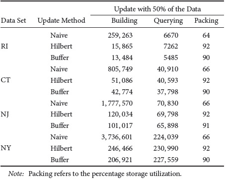
Figure 28.6 compares the construction cost for building R-trees and the resulting query performance in terms of I/Os for the naive sequential method for construction into R*-trees (labeled “naive”) and the newly developed buffer R*-tree method [26] (labeled “buffer”). An R-tree was constructed on the TIGER road data for each state and for each of four possible buffer sizes. The four buffer sizes were capable of storing 0, 600, 1250, and 5000 rectangles, respectively; buffer size 0 corresponds to the naive method, and the larger buffers correspond to the buffer method. The query performance of each resulting R-tree was measured by posing rectangle intersection queries using rectangles taken from TIGER hydrographic data. The results, depicted in Figure 28.6, show that buffer R*-trees, even with relatively small buffers, achieve a tremendous speedup in number of I/Os for construction without any worsening in query performance, compared with the naive method. The CPU costs of the two methods are comparable. The storage utilization of buffer R*-trees tends to be in the 90% range, as opposed to roughly 70% for the naive method.

Bottom-up methods can build R-trees even more quickly and more compactly, but they generally do not support bulk dynamic operations, which are a big advantage of the buffer tree approach. Kamel et al. [97] develop a way to do bulk updates with Hilbert R-trees, but at a cost in terms of query performance. Table 28.1 compares dynamic update methods for the naive method, for buffer R-trees, and for Hilbert R-trees [97] (labeled “Hilbert”). A single R-tree was built for each of the four U.S. states, containing 50% of the road data objects for that state. Using each of the three algorithms, the remaining 50% of the objects were inserted into the R-tree, and the construction time was measured. Query performance was then tested as before. The results in Table 28.1 indicate that the buffer R*-tree and the Hilbert R-tree achieve a similar degree of packing, but the buffer R*-tree provides better update and query performance.

Arge et al. [99] introduce the priority R-tree, which provides guaranteed query performance of O(n^{1 − 1/d} + z) I/Os, similarly to the search structures in Section 28.4.1. This query performance is optimal in the worst case for linear-sized data structures. The priority R-tree uses a bulk loading to construct the tree, and it supports updates efficiently in the amortized sense.

28.4.3Bootstrapping for 2-D Diagonal Corner and Stabbing Queries

An obvious paradigm for developing an efficient dynamic EM data structure, given an existing data structure that works well when the problem fits into internal memory, is to “externalize” the internal memory data structure. If the internal memory data structure uses a binary tree, then a multiway tree such as a B-tree must be used instead. However, when searching a B-tree, it can be difficult to report the outputs in an output-sensitive manner. For example, in certain searching applications, each of the Θ(B) subtrees of a given node in a B-tree may contribute one item to the query output, and as a result each subtree may need to be explored (costing several I/Os) just to report a single output item.

Fortunately, we can sometimes achieve output-sensitive reporting by augmenting the data structure with a set of filtering substructures, each of which is a data structure for a smaller version of the same problem. We refer to this approach, which we explain shortly in more detail, as the bootstrapping paradigm. Each substructure typically needs to store only O(B2) items and to answer queries in I/Os, where Z′ is the number of items reported. A substructure can even be static if it can be constructed in O(B) I/Os, since we can keep updates in a separate buffer and do a global rebuilding in O(B) I/Os whenever there are Θ(B) updates. Such a rebuilding costs O(1) I/Os (amortized) per update. We can often remove the amortization and make it worst case using the weight-balanced B-trees of Section 28.3.2 as the underlying B-tree structure.

Arge and Vitter [54] first uncovered the bootstrapping paradigm while designing an optimal dynamic EM data structure for diagonal corner two-sided 2-D queries (see Figure 28.5a) that meets all three design criteria for online data structures listed in Section 28.1.2. Diagonal corner two-sided queries are equivalent to stabbing queries, which have the following form: “Given a set of one-dimensional intervals, report all the intervals ‘stabbed’ by the query value x” (i.e., report all intervals that contain x). A diagonal corner query x on a set of 2-D points {(a1, b2), (a2, b2), …} is equivalent to a stabbing query x on the set of closed intervals {[a1, b2], [a2, b2], …}.

The EM data structure for stabbing queries is a multiway version of the well-known interval tree data structure [59,60] for internal memory, which supports stabbing queries in O(log N + Z) CPU time and updates in O(log N) CPU time and uses O(N) space. We can externalize it by using a weight-balanced B-tree as the underlying base tree, where the nodes have degree . Each node in the base tree corresponds in a natural way to a one-dimensional range of x-values; its children correspond to subranges called slabs, and the contiguous sets of slabs are called multislabs, as in Section 28.2 for a similar batched problem. Each input interval is stored in the lowest node v in the base tree whose range completely contains the interval. The interval is decomposed by v’s slabs into at most three pieces: the middle piece that completely spans one or more slabs of v, the left end piece that partially protrudes into a slab of v, and the right end piece that partially protrudes into another slab of v, as shown in Figure 28.7. The three pieces are stored in substructures of v. In the example in Figure 28.7, the middle piece is stored in a list associated with the multislab it spans (corresponding to the contiguous range of slabs 3–5), the left end piece is stored in a one-dimensional list for slab 2 ordered by left endpoint, and the right end piece is stored in a one-dimensional list for slab 6 ordered by right endpoint.

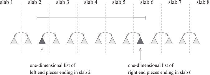
Figure 28.7Internal node v of the EM priority search tree, for $B = 64$ $B = 64$ with slabs. Node v is the lowest node in the tree completely containing the indicated interval. The middle piece of the interval is stored in the multislab list corresponding to slabs 3–5. (The multislab lists are not pictured.) The left and right end pieces of the interval are stored in the left-ordered list of slab 2 and the right-ordered list of slab 6, respectively.

Given a query value x, the intervals stabbed by x reside in the substructures of the nodes of the base tree along the search path from the root to the leaf for x. For each such node v, we consider each of v’s multislabs that contains x and report all the intervals in the multislab list. We also walk sequentially through the right-ordered list and left-ordered list for the slab of v that contains x, reporting intervals in an output-sensitive way.

The big problem with this approach is that we have to spend at least one I/O per multislab containing x, regardless of how many intervals are in the multislab lists. For example, there may be Θ(B) such multislab lists, with each list containing only a few stabbed intervals (or worse yet, none at all). The resulting query performance will be highly nonoptimal. The solution, according to the bootstrapping paradigm, is to use a substructure in each node consisting of an optimal static data structure for a smaller version of the same problem; a good choice is the corner data structure developed by Kanellakis et al. [72]. The corner substructure in this case is used to store all the intervals from the “sparse” multislab lists, namely those that contain fewer than B intervals, and thus the substructure contains only O(B2) intervals. When visiting node v, we access only v’s nonsparse multislab lists, each of which contributes Z′ ≥ B intervals to the output, at an output-sensitive cost of O(Z′/B) I/Os, for some Z′. The remaining Z′′ stabbed intervals stored in v can be found by a single query to v’s corner substructure, at a cost of I/Os. Since there are O(log_B N) nodes along the search path in the base tree, the total collection of Z stabbed intervals is reported in O(log_B N + z) I/Os, which is optimal. Using a weight-balanced B-tree as the underlying base tree allows the static substructures to be rebuilt in worst-case optimal I/O bounds.

Stabbing queries are important because, when combined with one-dimensional range queries, they provide a solution to dynamic interval management, in which one-dimensional intervals can be inserted and deleted, and intersection queries can be performed. These operations support indexing of one-dimensional constraints in constraint databases. Other applications of stabbing queries arise in graphics and GIS. For example, Chiang and Silva [100] apply the EM interval tree structure to extract at query time the boundary components of the isosurface (or contour) of a surface. A data structure for a related problem, which in addition has optimal output complexity, appears in Reference 101. The above bootstrapping approach also yields dynamic EM segment trees with optimal query and update bound and O(n log_B N)-block space usage.

28.4.4Bootstrapping for Three-Sided Orthogonal 2-D Range Search

Arge et al. [102] provide another example of the bootstrapping paradigm by developing an optimal dynamic EM data structure for three-sided orthogonal 2-D range searching (see Figure 28.5c) that meets all three design Criteria O1–O3. In internal memory, the optimal structure is the priority search tree [103], which answers three-sided range queries in O(log N + Z) CPU time, does updates in O(log N) CPU time, and uses O(N) space. The EM structure of Arge et al. [102] is an externalization of the priority search tree, using a weight-balanced B-tree as the underlying base tree. Each node in the base tree corresponds to a one-dimensional range of x-values, and its Θ(B) children correspond to subranges consisting of vertical slabs. Each node v contains a small substructure called a child cache that supports three-sided queries. Its child cache stores the “Y-set” Y (w) for each of the Θ(B) children w of v. The Y-set Y (w) for child w consists of the highest Θ(B) points in w’s slab that are not already stored in the child cache of some ancestor of v. There are thus a total of Θ(B2) points stored in v’s child cache.

We can answer a three-sided query of the form [x1, x2] × [y1, +∞) by visiting a set of nodes in the base tree, starting with the root. For each visited node v, we pose the query [x1, x2] × [y1, +∞) to v’s child cache and output the results. The following rules are used to determine which of v’s children to visit. We visit v’s child w (see Figure 28.8) if either

1.w is along the leftmost search path for x1 or the rightmost search path for x2 in the base tree, or

2.the entire Y-set Y (w) is reported when v’s child cache is queried.

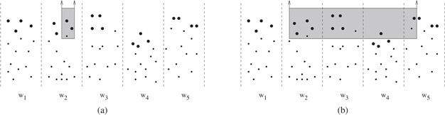
Figure 28.8Internal node v of the EM priority search tree, with slabs (children) w1, w2, …, w5. The Y-sets of each child, which are stored collectively in v’s child cache, are indicated by the bold points. (a) The three-sided query is completely contained in the x-range of w2. The relevant (bold) points are reported from v’s child cache, and the query is recursively answered in w2. (b) The three-sided query spans several slabs. The relevant (bold) points are reported from v’s child cache, and the query is recursively answered in w2, w3, and w5. The query is not extended to w4 in this case because not all of its Y-set Y (w4) (stored in v’s child cache) satisfies the query, and as a result, none of the points stored in w4’s subtree can satisfy the query.

There are O(log_B N) nodes w that are visited because of rule 1. When rule 1 is not satisfied, rule 2 provides an effective filtering mechanism to guarantee output-sensitive reporting. The I/O cost for initially accessing a child node w can be charged to the Θ(B) points of Y(w) reported from v’s child cache; conversely, if not all of Y (w) is reported, then the points stored in w’s subtree will be too low to satisfy the query, and there is no need to visit w (see Figure 28.8b). Provided that each child cache can be queried in O(1) I/Os plus the output-sensitive cost to output the points satisfying the query, the resulting overall query time is O(log_B N + z), as desired.

All that remains is to show how to query a child cache in a constant number of I/Os, plus the output-sensitive cost. Arge et al. [102] provide an elegant and optimal static data structure for three-sided range search, which can be used in the EM priority search tree described earlier to implement the child caches of size O(B2). The static structure is a persistent B-tree optimized for batched construction. When used for O(B2) points, it occupies O(B) blocks, can be built in O(B) I/Os, and supports three-sided queries in I/Os per query, where Z′ is the number of points reported. The static structure is so simple that it may be useful in practice on its own.

Both the three-sided structure developed by Arge et al. [102] and the structure for two-sided diagonal queries discussed in Section 28.4.3 satisfy Criteria O1–O3 of Section 28.1.2. So in a sense, the three-sided query structure subsumes the diagonal two-sided structure, since three-sided queries are more general. However, diagonal two-sided structure may prove to be faster in practice, because in each of its corner substructures, the data accessed during a query are always in contiguous blocks, whereas the static substructures used for three-sided search do not guarantee block contiguity. Empirical work is ongoing to evaluate the performance of these data structures.

On a historical note, earlier work on two-sided and three-sided queries was done by Ramaswamy and Subramanian [104] using the notion of path caching; their structure met Criterion O1 but had higher storage overheads and amortized and/or nonoptimal update bounds. Subramanian and Ramaswamy [73] subsequently developed the p-range tree data structure for three-sided queries, with optimal linear disk space and nearly optimal query and amortized update bounds.

28.4.5General Orthogonal 2-D Range Search

The dynamic data structure for three-sided range searching can be generalized using the filtering technique of Chazelle [8] to handle general four-sided queries with optimal I/O query bound O(log_B N + z) and optimal disk space usage [102]. The update bound becomes , which may not be optimal.

The outer level of the structure is a balanced (log_B N + 1)-way 1-D search tree with Θ(n) leaves, oriented, say, along the x-dimension. It therefore has about levels. At each level of the tree, each input point is stored in four substructures (described later) that are associated with the particular tree node at that level that spans the x-value of the point. The space and update bounds quoted above follow from the fact that the substructures use linear space and can be updated in O(log_B N) I/Os.

To search for the points in a four-sided query rectangle [x1, x2] × [y1, y2], we decompose the four-sided query in the following natural way into two three-sided queries, a stabbing query, and log_BN − 1 list traversals. We find the lowest node v in the tree whose x-range contains [x1, x2]. If v is a leaf, we can answer the query in a single I/O. Otherwise we query the substructures stored in those children of v whose x-ranges intersect [x1, x2]. Let 2 ≤ k ≤ log_BN + 1 be the number of such children. The range query when restricted to the leftmost such child of v is a three-sided query of the form [x1, +∞] × [y1, y2], and when restricted to the rightmost such child of v, the range query is a three-sided query of the form [−∞, x2] × [y1, y2]. Two of the substructures at each node are devoted for three-sided queries of these types; using the linear-sized data structures of Arge et al. [102] in Section 28.4.4, each such query can be done in O(log_B N + z) I/Os.

For the k − 2 intermediate children of v, their x-ranges are completely contained inside the x-range of the query rectangle, and thus we need only do k − 2 list traversals in y-order and retrieve the points whose y-values are in the range [y1, y2]. If we store the points in each node in y-order (in the third type of substructure), the Z′ output points from a node can be found in I/Os, once a starting point in the linear list is found. We can find all k − 2 starting points via a single query to a stabbing query substructure S associated with v. (This structure is the fourth type of substructure.) For each two y-consecutive points (a_i, b_i) and (a_{i + 1}, b_{i + 1}) associated with a child of v, we store the y-interval [b_i, b_{i + 1}] in S. Note that S contains intervals contributed by each of the log_BN + 1 children of v. By a single stabbing query with query value y1, we can thus identify the k − 2 starting points in only O(log_B N) I/Os [54], as described in Section 28.4.3. (We actually get starting points for all the children of v, not just the k − 2 ones of interest, but we can discard the starting points we don’t need.) The total number of I/Os to answer the range query is thus O(log_B N + z), which is optimal.

28.4.6Lower Bounds for Orthogonal Range Search

We mentioned in Section 28.4 that Subramanian and Ramaswamy [73] prove that no EM data structure for 2-D range searching can achieve design Criterion O1 of Section 28.1.2 using less than disk blocks, even if we relax the criterion and allow I/Os per query, for any constant c. The result holds for an EM version of the pointer machine model, based upon the approach of Chazelle [105] for the internal memory model.

Hellerstein et al. [106] consider a generalization of the layout-based lower bound argument of Kanellakis et al. [72] for studying the trade-off between disk space usage and query performance. They develop a model for indexability, in which an “efficient” data structure is expected to contain the Z output points to a query compactly within blocks. One shortcoming of the model is that it considers only data layout and ignores the search component of queries, and thus it rules out the important filtering paradigm discussed earlier in Section 28.4. For example, it is reasonable for any query to perform at least log_BN I/Os, so if the output size Z is at most B, a data structure may still be able to satisfy Criterion O1 even if the output is contained within O(log_B N) blocks rather than O(z) = O(1) blocks. Arge et al. [102] modify the model to rederive the same nonlinear space lower bound of Subramanian and Ramaswamy [73] for 2-D range searching by considering only output sizes Z larger than (log_B N)cB, for which the number of blocks allowed to hold the outputs is . This approach ignores the complexity of how to find the relevant blocks, but as mentioned in Section 28.4.5, the authors separately provide an optimal 2-D range search data structure that uses the same amount of disk space and does queries in the optimal O(log_B N + z) I/Os. Thus, despite its shortcomings, the indexability model is elegant and can provide much insight into the complexity of blocking data in EM. Further results in this model appear in References 107 and 108.

One intuition from the indexability model is that less disk space is needed to efficiently answer 2-D queries when the queries have bounded aspect ratio (i.e., when the ratio of the longest side length to the shortest side length of the query rectangle is bounded). An interesting question is whether R-trees and the linear-space structures of Sections 28.4.1 and 28.4.2 can be shown to perform provably well for such queries. Another interesting scenario is where the queries correspond to snapshots of the continuous movement of a sliding rectangle.

When the data structure is restricted to contain only a single copy of each point, Kanth and Singh [75] show for a restricted class of index-based trees that d-dimensional range queries in the worst case require Ω(n^{1 − 1/d} + z) I/Os, and they provide a data structure with a matching bound. Another approach to achieve the same bound is the cross tree data structure [74] mentioned in Section 28.4.1, which in addition supports the operations of cut and concatenate.

28.5Related Problems

For other types of range searching, such as in higher dimensions and for nonorthogonal queries, different filtering techniques are needed. So far, relatively little work has been done, and many open problems remain.

Vengroff and Vitter [109] developed the first theoretically near-optimal EM data structure for static three-dimensional orthogonal range searching. They create a hierarchical partitioning in which all the points that dominate a query point are densely contained in a set of blocks. Compression techniques are needed to minimize disk storage. If we use (B log n)-approximate boundaries rather than B-approximate boundaries, queries can be done in O(log_B N + z) I/Os, which is optimal, and the space usage is disk blocks to support (3 + k)-sided 3-D range queries, in which k of the dimensions (0 ≤ k ≤ 3) have finite ranges. The result also provides optimal O(log N + Z)-time query performance for three-sided 3-D queries in the (internal memory) RAM model, but using O(N log N) space.

Afshani [110] introduced the first optimal 3-D structure for dominance queries, and Afshani et al. [111] developed structures for range queries in higher dimensions.

By the reduction in Reference 112, a data structure for three-sided 3-D queries also applies to 2-D homothetic range search, in which the queries correspond to scaled and translated (but not rotated) transformations of an arbitrary fixed polygon. An interesting special case is “fat” orthogonal 2-D range search, where the query rectangles are required to have bounded aspect ratio. For example, every rectangle with bounded aspect ratio can be covered by two overlapping squares. An interesting open problem is to develop linear-sized optimal data structures for fat orthogonal 2-D range search. By the reduction, one possible approach would be to develop optimal linear-sized data structures for three-sided 3-D range search.

Agarwal et al. [113] consider halfspace range searching, in which a query is specified by a hyperplane and a bit indicating one of its two sides, and the output of the query consists of all the points on that side of the hyperplane. They give various data structures for half-space range searching in two, three, and higher dimensions, including one that works for simplex (polygon) queries in two dimensions, but with a higher query I/O cost. They have subsequently improved the storage bounds for half-space range queries in two dimensions to obtain an optimal static data structure satisfying Criteria O1 and O2 of Section 28.1.2.

The number of I/Os needed to build the data structures for 3-D orthogonal range search and half-space range search is rather large (more than Ω(N)). Still, the structures shed useful light on the complexity of range searching and may open the way to improved solutions. An open problem is to design efficient construction and update algorithms and to improve upon the constant factors.

Cheng et al. [114,115] look at a model of uncertainty, in which the location of each data point is given by a probability distribution, and give efficient indexes for range queries and join queries.

An interesting model related to range searching involves pattern matching in string data, and there has been great interest recently in EM algorithms for string processing. Chien et al. [116] derive a duality relation that links the number of I/O steps and the space bound for range searching to the corresponding measures for text indexing. Hon et al. [117] provide a formal framework for efficiently retrieving the most relevant occurrences satisfying a query pattern. Their index takes linear space and can be reduced to sublinear space by exploiting the compressibility of the data. Their work is an example of a compressed data structure, in which the goal is to construct a search structure whose size is roughly comparable to the size of the input in compressed format, but which can still be queried directly in an efficient manner. Other work on compressed data structures appears in Vitter [1].

Callahan et al. [118] develop dynamic EM data structures for several online problems in d dimensions. For any fixed ε > 0, they can find an approximate nearest neighbor of a query point (within a 1 + ε factor of optimal) in O(log_B N) I/Os; insertions and deletions can also be done in O(log_B N) I/Os. They use a related approach to maintain the closest pair of points; each update costs O(log_B N) I/Os. Govindarajan et al. [67] achieve the same bounds for closest pair by maintaining a well-separated pair decomposition. For finding nearest neighbors and approximate nearest neighbors, two other approaches are partition trees [113,119] and locality-sensitive hashing [120]. Numerous other data structures have been developed for range queries and related problems on spatial data. We refer to References 32, 88, and 89 for a broad survey.

28.6Dynamic and Kinetic Data Structures

In this section, we consider two scenarios where data items change: dynamic (in which items are inserted and deleted) and kinetic (in which the data items move continuously along specified trajectories). In both cases, queries can be done at any time. It is often useful for kinetic data structures to allow insertions and deletions; for example, if the trajectory of an item changes, we must delete the old trajectory and insert the new one.

28.6.1Logarithmic Method for Decomposable Search Problems

In previous sections, we’ve already encountered several dynamic data structures for the problems of dictionary lookup and range search. In Section 28.4, we saw how to develop optimal EM range search data structures by externalizing some known internal memory data structures. The key idea was to use the bootstrapping paradigm, together with weight-balanced B-trees as the underlying data structure, in order to consolidate several static data structures for small instances of range searching into one dynamic data structure for the full problem. The bootstrapping technique is specific to the particular data structures involved. In this section, we look at another technique that is based upon the properties of the problem itself rather than upon that of the data structure.

We call a problem decomposable if we can answer a query by querying individual subsets of the problem data and then computing the final result from the solutions to each subset. Dictionary search and range searching are obvious examples of decomposable problems. Bentley developed the logarithmic method [121,122] to convert efficient static data structures for decomposable problems into general dynamic ones. In the internal memory setting, the logarithmic method consists of maintaining a series of static substructures, at most one each of size 1, 2, 4, 8, … When a new item is inserted, it is initialized in a substructure of size 1. If a substructure of size 1 already exists, the two substructures are combined into a single substructure of size 2. If there is already a substructure of size 2, they in turn are combined into a single substructure of size 4, and so on. For the current value of N, it is easy to see that the kth substructure (i.e., of size 2k) is present exactly when the kth bit in the binary representation of N is 1. Since there are at most log N substructures, the search time bound is log N times the search time per substructure. As the number of items increases from 1 to N, the kth structure is built a total of N/2k times (assuming N is a power of 2). If it can be built in O(2k) time, the total time for all insertions and all substructures is thus O(N log N), making the amortized insertion time O(log N). If we use up to three substructures of size 2k at a time, we can do the reconstructions in advance and convert the amortized update bounds to worst case [122].

In the EM setting, in order to eliminate the dependence upon the binary logarithm in the I/O bounds, the number of substructures must be reduced from log N to log_BN, and thus the maximum size of the kth substructure must be increased from 2k to Bk. As the number of items increases from 1 to N, the kth substructure has to be built NB/Bk times (when N is a power of B), each time taking $O (B^{k} (\log_{B} N) / B)$ $O (B^{k} (\log_{B} N) / B)$ I/Os. The key point is that the extra factor of B in the numerator of the first term is cancelled by the factor of B in the denominator of the second term, and thus the resulting total insertion time over all N insertions and all log_BN structures is I/Os, which is I/Os amortized per insertion. By global rebuilding, we can do deletions in O(log_B N) I/Os amortized. As in the internal memory case, the amortized updates can typically be made worst case.

Arge and Vahrenhold [123] obtain I/O bounds for dynamic point location in general planar subdivisions similar to those of Reference 62, but without use of level-balanced trees. Their method uses a weight-balanced base structure at the outer level and a multislab structure for storing segments similar to that of Arge and Vitter [54] described in Section 28.4.3. They use the logarithmic method to construct a data structure to answer vertical rayshooting queries in the multislab structures. The method relies upon a total ordering of the segments, but such an ordering can be changed drastically by a single insertion. However, each substructure in the logarithmic method is static (until it is combined with another substructure), and thus a static total ordering can be used for each substructure. The authors show by a type of fractional cascading that the queries in the log_BN substructures do not have to be done independently, which saves a factor of log_B N in the I/O cost, but at the cost of making the data structures amortized instead of worst case.

Agarwal et al. [55] apply the logarithmic method (in both the binary form and B-way variant) to get EM versions of kd-trees, BBD trees, and BAR trees.

28.6.2Continuously Moving Items

Early work on temporal data generally concentrated on time-series or multiversion data [50]. A question of growing interest in this mobile age is how to store and index continuously moving items, such as mobile telephones, cars, and airplanes, using kinetic data structures [124–126]. There are two main approaches to storing moving items. The first technique is to use the same sort of data structure as for nonmoving data, but to update it whenever items move sufficiently far so as to trigger important combinatorial events that are relevant to the application at hand [127]. For example, an event relevant for range search might be triggered when two items move to the same horizontal displacement (which happens when the x-ordering of the two items is about to switch). A different approach is to store each item’s location and speed trajectory, so that no updating is needed as long as the item’s trajectory plan does not change. Such an approach requires fewer updates, but the representation for each item generally has higher dimension, and the search strategies are therefore less efficient.

Kollios et al. [128] developed a linear-space indexing scheme for moving points along an 1-D line, based upon the notion of partition trees. Their structure supports a variety of range search and approximate nearest-neighbor queries. For example, given a range and time, the points in that range at the indicated time can be retrieved in O(n^1/2+ε + k) I/Os, for arbitrarily small ε > 0. Updates require $O ((\log n)^{2})$ $O ((\log n)^{2})$ I/Os. Agarwal et al. [119] extend the approach to handle range searches in two dimensions, and they improve the update bound to $O ((\log_{B} n)^{2})$ $O ((\log_{B} n)^{2})$ I/Os. They also propose an event-driven data structure with the same query times as the range search data structure of Arge and Vitter [102] discussed in Section 28.4.5, but with the potential need to do many updates. A hybrid data structure combining the two approaches permits a trade-off between query performance and update frequency.

R-trees offer a practical generic mechanism for storing multidimensional points and are thus a natural alternative for storing mobile items. One approach is to represent time as a separate dimension and to cluster trajectories using the R-tree heuristics. However, the orthogonal nature of the R-tree does not lend itself well to diagonal trajectories. For the case of points moving along linear trajectories, Šaltenis et al. [125] build the R-tree upon only the spatial dimensions, but parameterize the bounding box coordinates to account for the movement of the items stored within. They maintain an outer approximation of the true bounding box, which they periodically update to refine the approximation. Agarwal and Har-Peled [129] show how to maintain a provably good approximation of the minimum bounding box with need for only a constant number of refinement events. Further discussion of kinetic data structures, primarily for internal memory, appears in Chapter 24.

28.7Conclusion

In this chapter, we have surveyed several useful paradigms and techniques for the design and implementation of efficient data structures for EM. A variety of interesting challenges remain in geometric search applications, such as methods for high-dimensional and nonorthogonal range searches as well as the analysis of R-trees and linear-space methods for typical case scenarios. A continuing goal is to translate theoretical gains into observable improvements in practice. For some of the problems that can be solved optimally up to a constant factor, the constant overhead is too large for the algorithm to be of practical use, and simpler approaches are needed.

Acknowledgments

The author thanks the members of the Center for Geometric Computing at Duke University for helpful comments and suggestions. This work was supported in part by the Army Research Office through grant DAAD19-03-1-0321, and by the National Science Foundation through research grants CCR-9877133, CCR-0082986, CCF-0328013, IIS-0415097, CCF-0621457, and CCF-1017623.

References

1.J. S. Vitter. Algorithms and data structures for external memory. Foundations and Trends in Theoretical Computer Science. Now Publishers, Hanover, MA, 2008.

2.J. S. Vitter and E. A. M. Shriver. Algorithms for parallel memory I: Two-level memories. Algorithmica, 12(2–3):110–147, 1994.

3.P. M. Chen, E. K. Lee, G. A. Gibson, R. H. Katz, and D. A. Patterson. RAID: High-performance, reliable secondary storage. ACM Computing Surveys, 26(2):145–185, 1994.

4.L. Hellerstein, G. Gibson, R. M. Karp, R. H. Katz, and D. A. Patterson. Coding techniques for handling failures in large disk arrays. Algorithmica, 12(2–3):182–208, 1994.

5.R. D. Barve, E. A. M. Shriver, P. B. Gibbons, B. K. Hillyer, Y. Matias, and J. S. Vitter. Modeling and optimizing I/O throughput of multiple disks on a bus. In Proceedings of the ACM SIGMETRICS Joint International Conference on Measurement and Modeling of Computer Systems, pages 83–92, Atlanta, GA, May 1999.

6.C. Ruemmler and J. Wilkes. An introduction to disk drive modeling. IEEE Computer, 23(3): 17–28, 1994.

7.E. A. M. Shriver, A. Merchant, and J. Wilkes. An analytic behavior model for disk drives with readahead caches and request reordering. In Proceedings of ACM SIGMETRICS Joint International Conference on Measurement and Modeling of Computer Systems, pages 182–191, June 1998.

8.B. Chazelle. Filtering search: A new approach to query-answering. SIAM Journal on Computing, 15:703–724, 1986.

9.J. S. Vitter. External memory algorithms and data structures: Dealing with massive data. ACM Computing Surveys, 33(2):209–271, 2001.

10.M. T. Goodrich, J.-J. Tsay, D. E. Vengroff, and J. S. Vitter. External-memory computational geometry. In Proceedings of the IEEE Symposium on Foundations of Computer Science, volume 34, pages 714–723, Palo Alto, IEEE Computer Society Press, November 1993.

11.B. Zhu. Further computational geometry in secondary memory. In Proceedings of the International Symposium on Algorithms and Computation, volume 834 of LNCS, pages 514–522, Springer, 1994.

12.L. Arge, D. E. Vengroff, and J. S. Vitter. External-memory algorithms for processing line segments in geographic information systems. Algorithmica, 47(1):1–25, 2007.

13.L. Arge, O. Procopiuc, S. Ramaswamy, T. Suel, and J. S. Vitter. Theory and practice of I/O-efficient algorithms for multidimensional batched searching problems. In Proceedings of the ACM-SIAM Symposium on Discrete Algorithms, volume 9, pages 685–694, 1998.

14.A. Crauser, P. Ferragina, K. Mehlhorn, U. Meyer, and E. A. Ramos. I/O-optimal computation of segment intersections. In J. Abello and J. S. Vitter, editors, External Memory Algorithms and Visualization, DIMACS Series in Discrete Mathematics and Theoretical Computer Science, pages 131–138. American Mathematical Society Press, Providence, RI, 1999.

15.A. Crauser, P. Ferragina, K. Mehlhorn, U. Meyer, and E. A. Ramos. Randomized external-memory algorithms for line segment intersection and other geometric problems. International Journal of Computational Geometry & Applications, 11(3):305–337, 2001.

16.J. R. Driscoll, N. Sarnak, D. D. Sleator, and R. E. Tarjan. Making data structures persistent. Journal of Computer and System Sciences, 38:86–124, 1989.

17.W. Dittrich, D. A. Hutchinson, and A. Maheshwari. Blocking in parallel multisearch problems. Theoretical Computer Science, 34(2):145–189, 2001.

18.R. Tamassia and J. S. Vitter. Optimal cooperative search in fractional cascaded data structures. Algorithmica, 15(2):154–171, 1996.

19.D. G. Kirkpatrick and R. Seidel. The ultimate planar convex hull algorithm? SIAM Journal on Computing, 15:287–299, 1986.

20.K. L. Clarkson and P. W. Shor. Applications of random sampling in computational geometry, II. Discrete and Computational Geometry, 4:387–421, 1989.

21.M. de Berg, M. van Kreveld, M. Overmars, and O. Schwarzkopf. Computational Geometry Algorithms and Applications. Springer, Berlin, 1997.

22.F. P. Preparata and M. I. Shamos. Computational Geometry. Springer, Berlin, 1985.

23.Y.-J. Chiang. Experiments on the practical I/O efficiency of geometric algorithms: Distribution sweep vs. plane sweep. Computational Geometry: Theory and Applications, 8(4):211–236, 1998.

24.L. Arge, O. Procopiuc, S. Ramaswamy, T. Suel, and J. S. Vitter. Scalable sweeping-based spatial join. In Proceedings of the International Conference on Very Large Databases, volume 24, pages 570–581, New York, Morgan Kaufmann, August 1998.

25.J. M. Patel and D. J. DeWitt. Partition based spatial-merge join. In Proceedings of the ACM SIGMOD International Conference on Management of Data, pages 259–270, ACM Press, June 1996.

26.L. Arge, K. H. Hinrichs, J. Vahrenhold, and J. S. Vitter. Efficient bulk operations on dynamic R-trees. Algorithmica, 33(1):104–128, 2002.

27.TPIE User Manual and Reference, 1999. The manual and software distribution are available on the web at http://www.cs.duke.edu/TPIE/.

28.D. E. Vengroff and J. S. Vitter. I/O-efficient scientific computation using TPIE. In Proceedings of the NASA Goddard Conference on Mass Storage Systems, volume 5, pages II, 553–570, September 1996.

29.Topologically Integrated Geographic Encoding and Referencing system, TIGER/line1992datafiles, 1992. Available on the World-Wide Web at http://www.census.gov/geo/www/tiger/.

30.L. Arge, O. Procopiuc, S. Ramaswamy, T. Suel, J. Vahrenhold, and J. S. Vitter. A unified approach for indexed and non-indexed spatial joins. In Proceedings of the International Conference on Extending Database Technology, volume 7, Konstanz, Germany, ACM Press, March 2000.

31.R. D. Barve and J. S. Vitter. A theoretical framework for memory-adaptive algorithms. In Proceedings of the IEEE Symposium on Foundations of Computer Science, volume 40, pages 273–284, New York, IEEE Computer Society Press, October 1999.

32.V. Gaede and O. Günther. Multidimensional access methods. ACM Computing Surveys, 30(2):170–231, 1998.

33.R. Bayer and E. McCreight. Organization of large ordered indexes. Acta Informatica, 1:173–189, 1972.

34.D. Comer. The ubiquitous B-tree. ACM Computing Surveys, 11(2):121–137, 1979.

35.D. E. Knuth. Sorting and Searching, volume 3 of The Art of Computer Programming. Addison-Wesley, Reading, MA, 2nd edition, 1998.

36.A. C. Yao. On random 2–3 trees. Acta Informatica, 9:159–170, 1978.

37.R. A. Baeza-Yates. Expected behaviour of B⁺-trees under random insertions. Acta Informatica, 26(5):439–472, 1989.

38.K. Küspert. Storage utilization in B*-trees with a generalized overflow technique. Acta Informatica, 19:35–55, 1983.

39.R. A. Baeza-Yates and P.-A. Larson. Performance of B⁺-trees with partial expansions. IEEE Transactions on Knowledge and Data Engineering, 1(2):248–257, 1989.

40.B. Srinivasan. An adaptive overflow technique to defer splitting in B-trees. The Computer Journal, 34(5):397–405, 1991.

41.W. Litwin and D. Lomet. A new method for fast data searches with keys. IEEE Software, 4(2):16–24, 1987.

42.R. Baeza-Yates. Bounded disorder: The effect of the index. Theoretical Computer Science, 168:21–38, 1996.

43.D. Lomet. A simple bounded disorder file organization with good performance. ACM Transactions on Database Systems, 13(4):525–551, 1988.

44.P. E. O’Neil. The SB-tree. An index-sequential structure for high-performance sequential access. Acta Informatica, 29(3):241–265, 1992.

45.J. Rao and K. Ross. Cache conscious indexing for decision-support in main memory. In M. Atkinson et al., editors, Proceedings of the International Conference on Very Large Databases, volume 25, pages 78–89, Los Altos, CA, Morgan Kaufmann, 1999.

46.J. Rao and K. A. Ross. Making B⁺-trees cache conscious in main memory. In W. Chen, J. Naughton, and P. A. Bernstein, editors, Proceedings of the ACM SIGMOD International Conference on Management of Data, pages 475–486, Dallas, TX, 2000.

47.B. Becker, S. Gschwind, T. Ohler, B. Seeger, and P. Widmayer. An asymptotically optimal multiversion B-tree. VLDB Journal, 5(4):264–275, 1996.

48.P. J. Varman and R. M. Verma. An efficient multiversion access structure. IEEE Transactions on Knowledge and Data Engineering, 9(3):391–409, 1997.

49.M. C. Easton. Key-sequence data sets on indelible storage. IBM Journal of Research and Development, 30:230–241, 1986.

50.B. Salzberg and V. J. Tsotras. Comparison of access methods for time-evolving data. ACM Computing Surveys, 31:158–221, 1999.

51.P. L. Lehman and S. Bing Yao. Efficient locking for concurrent operations on B-trees. ACM Transactions on Database Systems, 6(4):650–670, 1981.

52.C. Mohan. ARIES/KVL: A key-value locking method for concurrency control of multiaction transactions on B-tree indices. In Proceedings of the International Conference on Very Large Databases, volume 16, pages 392–405, Brisbane, Australia, Morgan Kaufmann, August 1990.

53.D. B. Lomet and B. Salzberg. Concurrency and recovery for index trees. VLDB Journal, 6(3):224–240, 1997.

54.L. Arge and J. S. Vitter. Optimal external memory interval management. SIAM Journal on Computing, 32(6):1488–1508, 2003.

55.P. K. Agarwal, L. Arge, O. Procopiuc, and J. S. Vitter. A framework for index bulk loading and dynamization. In Proceedings of the International Colloquium on Automata, Languages, and Programming, volume 2076 of LNCS, pages 115–127, Crete, Greece, Springer, 2001.

56.N. Blum and K. Mehlhorn. On the average number of rebalancing operations in weight-balanced trees. Theoretical Computer Science, 11(3):303–320, July 1980.

57.J. Nievergelt and E. M. Reingold. Binary search tree of bounded balance. SIAM Journal on Computing, 2(1):33–43, 1973.

58.R. Grossi and G. F. Italiano. Efficient splitting and merging algorithms for order decomposable problems. Information and Computation, 154(1):1–33, 1999.

59.H. Edelsbrunner. A new approach to rectangle intersections, Part I. International Journal of Computer Mathematics, 13:209–219, 1983.

60.H. Edelsbrunner. A new approach to rectangle intersections, Part II. International Journal of Computer Mathematics, 13:221–229, 1983.

61.D.E. Willard and G.S. Lueker. Adding range restriction capability to dynamic data structures. Journal of the ACM, 32(3):597–617, 1985.

62.P. K. Agarwal, L. Arge, G. S. Brodal, and J. S. Vitter. I/O-efficient dynamic point location in monotone planar subdivisions. In Proceedings of the ACM-SIAM Symposium on Discrete Algorithms, volume 10, pages 11–20, ACM Press, 1999.

63.J. S. Vitter. Efficient memory access in large-scale computation. In Proceedings of the Symposium on Theoretical Aspects of Computer Science, volume 480 of LNCS, pages 26–41, Springer, Invited keynote paper, 1991.

64.L. Arge. The Buffer Tree: A technique for designing batched external data structures. Algorithmica, 37(1):1–24, 2003.

65.J. L. Bentley. Multidimensional divide and conquer. Communications of the ACM, 23(6):214–229, 1980.

66.Y.-J. Chiang, M. T. Goodrich, E. F. Grove, R. Tamassia, D. E. Vengroff, and J. S. Vitter. External-memory graph algorithms. In Proceedings of the ACM-SIAM Symposium on Discrete Algorithms, volume 6, pages 139–149, ACM Press, January 1995.

67.S. Govindarajan, T. Lukovszki, A. Maheshwari, and N. Zeh. I/O-efficient well-separated pair decomposition and its applications. Algorithmica, 45(4):385–614, 2006.

68.G. S. Brodal and J. Katajainen. Worst-case efficient external-memory priority queues. In Proceedings of the Scandinavian Workshop on Algorithmic Theory, volume 1432 of LNCS, pages 107–118, Stockholm, Sweden, Springer, July 1998.

69.K. Brengel, A. Crauser, P. Ferragina, and U. Meyer. An experimental study of priority queues in external memory. ACM Journal of Experimental Algorithmics, 5:17, 2000.

70.P. Sanders. Fast priority queues for cached memory. ACM Journal of Experimental Algorithmics, 5(7):1–25, 2000.

71.D. Hutchinson, A. Maheshwari, J-R. Sack, and R. Velicescu. Early experiences in implementing the buffer tree. In Proceedings of the Workshop on Algorithm Engineering, LNCS, Springer, 1997.

72.P. C. Kanellakis, S. Ramaswamy, D. E. Vengroff, and J. S. Vitter. Indexing for data models with constraints and classes. Journal of Computer and System Sciences, 52(3):589–612, 1996.

73.S. Subramanian and S. Ramaswamy. The P-range tree: A new data structure for range searching in secondary memory. In Proceedings of the ACM-SIAM Symposium on Discrete Algorithms, volume 6, pages 378–387, PUB, ACM Press, 1995.

74.R. Grossi and G. F. Italiano. Efficient cross-trees for external memory. In J. Abello and J. S. Vitter, editors, External Memory Algorithms and Visualization, DIMACS Series in Discrete Mathematics and Theoretical Computer Science, pages 87–106. American Mathematical Society Press, Providence, RI, 1999.

75.K. V. R. Kanth and A. K. Singh. Optimal dynamic range searching in non-replicating index structures. In Proceedings of the International Conference on Database Theory, volume 1540 of LNCS, pages 257–276, Springer, January 1999.

76.J. T. Robinson. The k-d–B-tree: A search structure for large multidimensional dynamic indexes. In Proceedings of the ACM Conference on Principles of Database Systems, volume 1, pages 10–18, ACM Press, 1981.

77.B. Seeger and H.-P. Kriegel. The buddy-tree: An efficient and robust access method for spatial data base systems. In Proceedings of the International Conference on Very Large Databases, volume 16, pages 590–601, Morgan Kaufmann, 1990.

78.G. Evangelidis, D. B. Lomet, and B. Salzberg. The hB^Π-tree: A multi-attribute index supporting concurrency, recovery and node consolidation. VLDB Journal, 6:1–25, 1997.

79.D. B. Lomet and B. Salzberg. The hB-tree: A multiattribute indexing method with good guaranteed performance. ACM Transactions on Database Systems, 15(4):625–658, 1990.

80.K. Hinrichs. Implementation of the grid file: Design concepts and experience. BIT, 25(4):569–592, 1985.

81.J. Nievergelt, H. Hinterberger, and K. C. Sevcik. The grid file: An adaptable, symmetric multi-key file structure. ACM Transactions on Database Systems, 9:38–71, 1984.

82.K.-Y. Whang and R. Krishnamurthy. Multilevel grid files—A dynamic hierarchical multidimensional file structure. In Proceedings of the International Symposium on Database Systems for Advanced Applications, pages 449–459, World Scientific Press, 1992.

83.I. Gargantini. An effective way to represent quadtrees. Communications of the ACM, 25(12):905–910, 1982.

84.I. Kamel, C. Faloutsos. Hilbert R-tree: An improved R-tree using fractals. In Proceedings of the International Conference on Very Large Databases, volume 20, pages 500–509, Morgan Kaufmann, 1994.

85.J. A. Orenstein and T. H. Merrett. A class of data structures for associative searching. In Proceedings of the ACM Conference on Principles of Database Systems, volume 3, pages 181–190, ACM Press, 1984.

86.D. J. Abel. A B⁺-tree structure for large quadtrees. Computer Vision, Graphics, and Image Processing, 27(1):19–31, 1984.

87.J. A. Orenstein. Redundancy in spatial databases. In Proceedings of the ACM SIGMOD International Conference on Management of Data, pages 294–305, Portland, OR, ACM Press, June 1989.

88.P. K. Agarwal and J. Erickson. Geometric range searching and its relatives. In B. Chazelle, J. E. Goodman, and R. Pollack, editors, Advances in Discrete and Computational Geometry, Volume 23 of Contemporary Mathematics, pages 1–56, American Mathematical Society Press, Providence, RI, 1999.

89.J. Nievergelt and P. Widmayer. Spatial data structures: Concepts and design choices. In M. van Kreveld, J. Nievergelt, T. Roos, and P. Widmayer, editors, Algorithmic Foundations of GIS, Volume 1340 of LNCS, pages 153–197, Springer, 1997.

90.A. Guttman. R-trees: A dynamic index structure for spatial searching. In Proceedings of the ACM SIGMOD International Conference on Management of Data, pages 47–57, ACM Press, 1984.

91.D. Greene. An implementation and performance analysis of spatial data access methods. In Proceedings of the IEEE International Conference on Data Engineering, volume 5, pages 606–615, IEEE Press, 1989.

92.N. Beckmann, H.-P. Kriegel, R. Schneider, and B. Seeger. The R*-tree: An efficient and robust access method for points and rectangles. In Proceedings of the ACM SIGMOD International Conference on Management of Data, pages 322–331, ACM Press, 1990.

93.M. de Berg, J. Gudmundsson, M. Hammar, and M. H. Overmars. On R-trees with low query complexity. Computational Geometry, 24(3):179–195, 2003.

94.P. K. Agarwal, M. de Berg, J. Gudmundsson, M. Hammar, and H. J. Haverkort. Box-trees and R-trees with near-optimal query time. Discrete and Computational Geometry, 28(3):291–312, 2002.

95.I. Kamel and C. Faloutsos. On packing R-trees. In Proceedings of the International ACM Conference on Information and Knowledge Management, volume 2, pages 490–499, ACM Press, 1993.

96.S. Berchtold, C. Böhm, and H-P. Kriegel. Improving the query performance of high-dimensional index structures by bulk load operations. In Proceedings of the International Conference on Extending Database Technology, volume 1377 of LNCS, pages 216–230, Springer, 1998.

97.I. Kamel, M. Khalil, and V. Kouramajian. Bulk insertion in dynamic R-trees. In Proceedings of the International Symposium on Spatial Data Handling, volume 4, pages 3B,31–42, Zurich: International Geographical Union, 1996.

98.J. van den Bercken, B. Seeger, and P. Widmayer. A generic approach to bulk loading multidimensional index structures. In Proceedings of the International Conference on Very Large Databases, volume 23, pages 406–415, 1997.

99.L. Arge, M. de Berg, H. J. Haverkort, and K. Yi. The priority R-tree: A practically efficient and worst-case optimal R-tree. ACM Transactions on Algorithms, 4(1):9, 2008.

100.Y.-J. Chiang and C. T. Silva. External memory techniques for isosurface extraction in scientific visualization. In J. Abello and J. S. Vitter, editors, External Memory Algorithms and Visualization, DIMACS Series in Discrete Mathematics and Theoretical Computer Science, pages 247–277, American Mathematical Society Press, Providence, RI, 1999.

101.P. K. Agarwal, L. Arge, T. M. Murali, K. Varadarajan, and J. S. Vitter. I/O-efficient algorithms for contour line extraction and planar graph blocking. In Proceedings of the ACM-SIAM Symposium on Discrete Algorithms, volume 9, pages 117–126, ACM Press, 1998.

102.L. Arge, V. Samoladas, and J. S. Vitter. Two-dimensional indexability and optimal range search indexing. In Proceedings of the ACM Conference on Principles of Database Systems, volume 18, pages 346–357, Philadelphia, PA, ACM Press, May–June 1999.

103.E. M. McCreight. Priority search trees. SIAM Journal on Computing, 14(2):257–276, 1985.

104.S. Ramaswamy and S. Subramanian. Path caching: A technique for optimal external searching. In Proceedings of the ACM Conference on Principles of Database Systems, volume 13, pages 25–35, Minneapolis, MN, ACM Press, 1994.

105.B. Chazelle. Lower bounds for orthogonal range searching: I. The reporting case. Journal of the ACM, 37(2):200–212, 1990.

106.J. M. Hellerstein, E. Koutsoupias, and C. H. Papadimitriou. On the analysis of indexing schemes. In Proceedings of the ACM Symposium on Principles of Database Systems, volume 16, pages 249–256, Tucson, AZ, ACM Press, May 1997.

107.E. Koutsoupias and D. S. Taylor. Tight bounds for 2-dimensional indexing schemes. In Proceedings of the ACM Symposium on Principles of Database Systems, volume 17, pages 52–58, Seattle, WA, ACM Press, June 1998.

108.V. Samoladas and D. Miranker. A lower bound theorem for indexing schemes and its application to multidimensional range queries. In Proceedings of the ACM Symposium on Principles of Database Systems, volume 17, pages 44–51, Seattle, WA, ACM Press, June 1998.

109.D. E. Vengroff and J. S. Vitter. Efficient 3-d range searching in external memory. In Proceedings of the ACM Symposium on Theory of Computing, volume 28, pages 192–201, Philadelphia, PA, ACM Press, May 1996.

110.P. Afshani. On dominance reporting in 3d. In Proceedings of the European Symposium on Algorithms, LNCS, pages 41–51. Springer, 2008.

111.P. Afshani, L. Arge, and K. D. Larsen. Orthogonal range reporting in three and higher dimensions. In Proceedings of the IEEE Symposium on Foundations of Computer Science, pages 149–158, IEEE Press, October 2009.

112.B. Chazelle and H. Edelsbrunner. Linear space data structures for two types of range search. Discrete and Computational Geometry, 2:113–126, 1987.

113.P. K. Agarwal, L. Arge, J. Erickson, P. G. Franciosa, and J. S. Vitter. Efficient searching with linear constraints. Journal of Computer and System Sciences, 61(2):194–216, October 2000.

114.R. Cheng, Y. Xia, S. Prabhakar, R. Shah, and J. S. Vitter. Efficient indexing methods for probabilistic threshold queries over uncertain data. In Proceedings of the International Conference on Very Large Databases, Toronto, CA, Morgan Kaufmann, August 2004.

115.R. Cheng, Y. Xia, S. Prabhakar, R. Shah, and J. S. Vitter. Efficient join processing over uncertain-valued attributes. In Proceedings of the International ACM Conference on Information and Knowledge Management, Arlington, VA, ACM Press, November 2006.

116.Y.-F. Chien, W.-K. Hon, R. Shah, and J. S. Vitter. Geometric Burrows-Wheeler transform: Linking range searching and text indexing. In Proceedings of the IEEE Data Compression Conference, pages 252–261, IEEE Press, 2008.

117.W.-K. Hon, R. Shah, S. V. Thankachan, and J. S. Vitter. Space-efficient frameworks for top-k string retrieval. Journal of the ACM, 61(2):9.1–9.36, 2014.

118.P. Callahan, M. T. Goodrich, and K. Ramaiyer. Topology B-trees and their applications. In Proceedings of the Workshop on Algorithms and Data Structures, volume 955 of LNCS, pages 381–392, Springer, 1995.

119.P. K. Agarwal, L. Arge, and J. Erickson. Indexing moving points. Journal of Computer and System Sciences, 66(1):207–243, 2003.

120.A. Gionis, P. Indyk, and R. Motwani. Similarity search in high dimensions via hashing. In Proceedings of the International Conference on Very Large Databases, volume 25, pages 78–89, Edinburgh, Scotland, Morgan Kaufmann, 1999.

121.J. L. Bentley and J. B. Saxe. Decomposable searching problems I: Static-to-dynamic transformations. Journal of Algorithms, 1(4):301–358, December 1980.

122.M. H. Overmars, The Design of Dynamic Data Structures. LNCS, Berlin: Springer, 1983.

123.L. Arge and J. Vahrenhold. I/O-efficient dynamic planar point location. Computational Geometry, 29(2):147–162, 2004.

124.D. Pfoser, C. S. Jensen, and Y. Theodoridis. Novel approaches to the indexing of moving object trajectories. In Proceedings of the International Conference on Very Large Databases, volume 26, pages 395–406, Cairo, Morgan Kaufmann, 2000.

125.S. Šaltenis, C. S. Jensen, S. T. Leutenegger, and M. A. Lopez. Indexing the positions of continuously moving objects. In W. Chen, J. Naughton, and P. A. Bernstein, editors, Proceedings of the ACM SIGMOD International Conference on Management of Data, pages 331–342, Dallas, Texas, ACM Press, 2000.

126.O. Wolfson. Moving objects information management: The database challenge. In A. Halevy and A. Gal, editors, Next Generation Information Technologies and Systems, volume 2382 of Lecture Notes in Computer Science, pages 75–89, Berlin Heidelberg, Springer, 2002.

127.J. Basch, L. J. Guibas, and J. Hershberger. Data structures for mobile data. Journal of Algorithms, 31:1–28, 1999.

128.G. Kollios, D. Gunopulos, and V. J. Tsotras. On indexing mobile objects. In Proceedings of the ACM Symposium on Principles of Database Systems, volume 18, pages 261–272, Morgan Kaufmann, 1999.

129.P. K. Agarwal and S. Har-Peled. Maintaining the approximate extent measures of moving points. In Proceedings of the ACM-SIAM Symposium on Discrete Algorithms, volume 12, pages 148–157, Washington, Morgan Kaufmann, January 2001.

*We use the notation log N to denote the binary (base 2) logarithm log2N. For bases other than 2, the base will be specified explicitly, as in the base-B logarithm log_B N.

..................Content has been hidden....................

You can't read the all page of ebook, please click here login for view all page.

Table of Contents for 28. Geometric and Spatial Data Structures in External Memory

Create new playlist

Sign In

Sign Up

Table of Contents for
28. Geometric and Spatial Data Structures in External Memory