34. Data Structures for Sets

Sets are a fundamental concept in computer science: the study of algorithms and data structures for maintaining them were among the earliest developments in data structures. Our focus will be on problems that involve maintaining a family $F$ $F$ of sets, where all sets are drawn from a universe U of elements. We do not assume that there is a particular natural order among the elements of U, and in particular do not focus on data structuring problems on sets where the operations explicitly assume such an order (e.g., priority queues). A base repertoire of actions is as follows:

\begin{array}{l} create () & Create a new empty set, add it to F and return the name of the set. \\ destroy (A) & If A = \emptyset then remove A from F . If A \neq \emptyset, flag an error. \\ insert (x, A) & Set A \leftarrow A \cup {x} . \\ delete (x, A) & Set A \leftarrow A - {x} . \end{array}}

$\begin{array}{l} create () & Create a new empty set, add it to F and return the name of the set. \\ destroy (A) & If A = \emptyset then remove A from F . If A \neq \emptyset, flag an error. \\ insert (x, A) & Set A \leftarrow A \cup {x} . \\ delete (x, A) & Set A \leftarrow A - {x} . \end{array}}$

(34.1)

The following operation is fundamental for data structuring problems involving sets in general, but plays only an auxiliary role in this chapter:

$member (x, A) Returns ‘true' if x \in A and ‘false' otherwise.$ $member (x, A) Returns ‘true' if x \in A and ‘false' otherwise.$	(34.2)

If we take only insert, delete and member, we get the dictionary problem, covered in Part III. The base repertoire plus member is essentially no more difficult, as it represents the problem of maintaining a collection of independent dictionaries over a common universe. In this chapter, we focus on adding operations to this base repertoire that take two or more sets as arguments. For example, we could consider the standard set-theoretic operations on two sets A and B:

A op B, op \in {\cup, \cap, -} .

$A op B, op \in {\cup, \cap, -} .$

A data structure may support only an enumerative form of these operations, whereby the result of A op B is, in essence, some kind of enumeration of the set A op B. This result may not be in the same representation as A or B, and so one may not be able operate on it (e.g., ((A op B) op C) may not involve just two executions of op). The complexity of the algorithms will generally be measured in terms of the following parameters:

\begin{aligned} \begin{aligned} n & = \sum_{A \in F} | A | (the total size of all sets in the family) \\ m & = | U | (the size of the universe) \\ k & = | F | (the number of sets in the family) \end{aligned} \end{aligned}

$\begin{aligned} \begin{aligned} n & = \sum_{A \in F} | A | (the total size of all sets in the family) \\ m & = | U | (the size of the universe) \\ k & = | F | (the number of sets in the family) \end{aligned} \end{aligned}$

(34.3)

34.1.1Models of Computation

The problems that we consider in this chapter have been studied on a variety of different computation models. The primary models for proving upper bounds are the pointer machine model and the random-access machine (RAM) model. The pointer machine [1–3] postulates a storage consisting of an unbounded collection of registers (or records) connected by pointers. Each register can contain an arbitrary amount of additional information, and no arithmetic is allowed to compute the address of a register. The processor has a constant number of (data and pointer) registers that it can manipulate directly, but all other temporary results must be held in the storage records. In particular, this means that to answer a query, the processor must either start from a pointer p into the data structure provided by the “user” or from one of the constant number of pointers it itself holds, and explore the data structure by following pointers starting from p.

The RAM model we use is a standard variant of the original RAM model [4], the word RAM model [5]. Briefly, the word RAM model uses the unit-cost criterion, and a word size of Θ(log n) bits, where $n = \sum_{S \in F} | S |$ $n = \sum_{S \in F} | S |$ .^* Clearly the word size should be at least log n + O(1) bits—otherwise one could not even address the amount of memory required to store $F$ $F$ . Nevertheless, there are instances where the solutions that result from the use of this model could be viewed as “cheating.” For example, we could have n = 2^Θ(|U|), in which case the word size would be Θ(|U|) bits, which would allow most set operations to be done in O(1) time by bitwise operations on a single word. The solutions that we discuss, however, do not exploit this fact. In the related cell probe model, the storage of the computer is modeled by cells numbered 0, 1, 2,…, each of which can store a number of O(log n) bits. The running time of an algorithm in this model is measured as just the number of words (cells) accessed during an operation. All other computations are free.

The arithmetic model, used primarily for proving lower bounds, was proposed by Fredman [6] and Yao [7]. We now give a somewhat simplified description of this model which conveys the essential aspects: the interested reader is referred to [8, section 7.2.3] for further details. In many cases of interest, it is useful to assume that the data structure operates on values from a set $M$ $M$ , which is a monoid. This means that $M = (M, +, 0)$ $M = (M, +, 0)$ is augmented with an associative and commutative operator + such that $M$ $M$ is closed under + and 0 is the identity element for +. The data structure is modeled as an collection of variables v0, v1,…, each of which can hold a value from $M$ $M$ and initially contains 0. After receiving the input to each operation, the algorithm executes a sequence of operations of the form $v_{i} \leftarrow$ $v_{i} \leftarrow$ INPUT, $v_{i} \leftarrow v_{j} + v_{k}$ $v_{i} \leftarrow v_{j} + v_{k}$ or OUTPUT $\leftarrow v_{i}$ $\leftarrow v_{i}$ . The algorithm must be correct for all choices of $M$ $M$ , thus in particular it cannot assume that the operator + is invertible. The cost of an algorithm in processing a sequence of operations is the total number of such instructions executed by it. The restriction that $M$ $M$ is a monoid (rather than say, a group) is partly for ease of proving lower bounds. However, known algorithms in this framework do not gain significant asymptotic speedups by exploiting stronger models (e.g., by using the fact that + is invertible in groups).

34.2Simple Randomized Set Representations

In this section we cover a simple, but general-purpose set representation due to [9,10]. In addition to the base repertoire (34.1), we wish to support:

A op B, op \in {\cup, \cap, -},

$A op B, op \in {\cup, \cap, -},$

as well as the following boolean operations:

$\begin{array}{rcl} equal (A, B) & Returns ‘true' if A = B and ‘false' otherwise. \end{array}$ $\begin{array}{rcl} equal (A, B) & Returns ‘true' if A = B and ‘false' otherwise. \end{array}$	(34.4)

$\begin{array}{rcl} subset (A, B) & Returns ‘true' if A \subseteq B and ‘false' otherwise. \end{array}$ $\begin{array}{rcl} subset (A, B) & Returns ‘true' if A \subseteq B and ‘false' otherwise. \end{array}$	(34.5)

This representation touches upon a topic of interest in its own right, that of the unique representation of sets, which can be defined as follows. We consider a class of representations that suffice to represent all subsets of a given universe U. However, we require that each set should have a a unique representation within that class. In particular the representation should be independent of the sequence of operations that created the set (e.g., a red-black tree representation is not unique). Unique representations have the desirable property that it is then possible to ensure that all instances of the same set within a family (including sets that are created as intermediate results in a computation) are represented by the same object within the data structure. This allows constant-time equality tests of two sets: just check if they are the same object! The difficulty, of course, is to combine unique representations with rapid updates.

This definition also applies to randomized algorithms, which may access a source of random bits while executing a query or update, and the uniqueness requirement here means that the choice of representation for a set depends solely upon the sequence of random bits that are output by the source. (If, as in practice, one uses a pseudo-random generator, then the representation for a given set depends only upon the seed used by the pseudo-random number generator.)

34.2.1The Hash Trie

We first weaken the notion of a unique representation, and speak about the unique representation of sets from a labeled universe. Here, we assume that the elements of the universe U are labeled with (not necessarily unique) b-bit strings, and for x ∈ U we denote its label by ℓ(x). In addition, we also have the notion of a labeled set A_y, where y is a sequence of ≤ b bits. Any labeled set A_y satisfies the property that for all x ∈ A_y, y is a prefix of ℓ(x).

Given a set from a labeled universe, one can of course use the well-known binary trie [11] to represent it. For the sake of precision we now define the binary trie, when used to represent a (labeled) set S_y:

•If |S_y| = 0 then the trie is empty.

•If |y| = b then the trie is a leaf node that contains a pointer to a linked list containing all elements of S_y.

•Otherwise, the trie comprises an internal node with an edge labeled 0 pointing to a binary trie for the set

S_{y 0} = {x \in S_{y} ∣ y 0 is a prefix of ℓ (x)}

$S_{y 0} = {x \in S_{y} ∣ y 0 is a prefix of ℓ (x)}$

and an edge labeled 1 pointing to a binary trie for the labeled set

S_{y 1} = {x \in S_{y} ∣ y 1 is a prefix of ℓ (x)}

$S_{y 1} = {x \in S_{y} ∣ y 1 is a prefix of ℓ (x)}$

A set S ⊆ U is represented as the labeled set S_Λ, where Λ denotes the empty string.

Consider a family $F$ $F$ of sets from a universe U and let each node in the resulting collection of tries represent a labeled set in the natural way. Then if two nodes represent labeled sets A_z and B_z, such that A_z = B_z (note that the label is the same) then the subtrees rooted at these nodes have an identical structure. One can then save space by ensuring that all sets in $F$ $F$ whose representations have instances of the set A_z point to a single instance of A_z. By consistently applying this principle, we will ensure that two sets S, T, S = T point to a single instance of S_Λ.

We now give an example. Let U = {a, b, c, d, e, f} and $F$ $F$ contain the sets X = {a, c, f}, Y = {c, d, e} and Z = {a, b, c, f}. Suppose that the elements of U are labeled as follows:

ℓ (a) = 001, ℓ (b) = 011, ℓ (c) = 010, ℓ (d) = 101, ℓ (e) = 110, ℓ (f) = 010

$ℓ (a) = 001, ℓ (b) = 011, ℓ (c) = 010, ℓ (d) = 101, ℓ (e) = 110, ℓ (f) = 010$

Without exploiting the unique representation property, we would get the representation in Figure 34.1(i), and by exploiting it and storing subtrees uniquely it we get the representation in Figure 34.1(ii). Updates now need to be done with a little care: one cannot, for example, add a new child to a node, as the subtree in which the node lies may be shared among a number of sets. The solution is to use nondestructive updates, namely, implementing updates by making a copy of the path from the leaf to be added/deleted to the name of the sets (cf. persistent data structures). Figure 34.1(iii) shows the state of the data structure after executing the commands insert(a, Y) and insert(b, X), which we now explain.

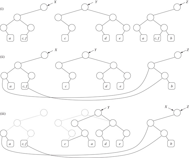
Figure 34.1Unique set representations.

First, let us consider the operation insert(a, Y). We need to insert a as a sibling of c in the trie for Y. Since the path from c up to the root of Y could potentially be shared by other sets, we do not modify the node that is the parent of c, instead making a copy of the entire path from c to the node that is the root of the representation of Y, as shown in the figure. The pointer for Y is then appropriately modified. The nodes that were previously part of the representation of Y (shown in dotted outline) are, in this example, not reachable as part of any set and may be cleared as part of a garbage-collection phase (they are not explicitly freed during the insertion). Now coming to insert(b, X), we proceed as before, and do not insert b directly as a sibling of (c, f) under X. However, before creating a new node with the leaves b and (c, f) as children, we check the data structure to see if such a node exists and find one (this is the node representing the set Z01). Therefore, we avoid creating this node. Continuing, we discover that all the nodes that we would have tried to create as part of this insertion already exist and therefore conclude that the sets X and Z are now the same (and hence their tries should be represented by the same node).

To support the reuse of existing nodes, a dictionary data structure that stores all nodes currently in the data structure is maintained. A node x with left child y and right child z is stored in this dictionary with the key 〈y, z〉 (either of y or z could be nil). Each insertion requires Θ(b) lookups or insertions into this dictionary. Avoiding this overhead is important, but in a randomized setting the dictionary can be implemented using dynamic perfect hashing, giving O(1) overhead. This idea is also used in practical implementations of functional programming languages such as LISP, and is referred to as hashed consing in that context.^*

In a randomized setting, the other problem, that of obtaining suitable labels, can also be solved easily. We simply let ℓ be a function chosen at random from a universal class of hash functions (cf. Chapter 9). By choosing $ℓ : U \to {1, \dots, n^{3}}$ $ℓ : U \to {1, \dots, n^{3}}$ (e.g.) we can ensure that the number of collisions, or pairs of distinct elements x, y in U with ℓ(x) = ℓ(y) is O(1) with a probability that tends to 1 as $n \to \infty$ $n \to \infty$ . This means that we can essentially ignore the possibility that there are more than a constant number of elements at the leaf of any trie. Clearly, labels are O(log n) bits long.

Note that we can ensure that both the lengths of the labels and the number of collisions stays under control as n changes, by simply rehashing whenever the value of n doubles or halves since the last rehash. We now analyze some parameters of this data structure. Clearly, equality testing takes O(1) time. Each insertion or deletion takes time and space proportional to the depth of the tries, which is O(log n). Both insertions and deletions may cause some nodes to become “garbage” (i.e., unreachable from any set)—these need to be compacted periodically, for example, when a rehash occurs. It is easy to verify that the amortized cost of rehashing and garbage collection is negligible. This gives parts (i) and (ii) of the following theorem; for part (iii) we refer the reader to [9, Chapter 8]:

Theorem 34.1

There is a data structure for a family of sets that:

i.Supports insert and delete in O(log n) amortized expected time and equality-testing in O(1) worst-case time;

ii.Uses O(n log n) space, and

iii.Given two sets A and B, supports the constructive version of A op B for op ∈ {∪, ∩, − ,⊆} in O(|S2|(1 + log (S3/S2) amortized expected time, where S2 and S3 are the middle and largest sets of A − B, B − A and A ∩ B.

Remark 34.1

Note that a fairly naive bound for an operation A op B, for op ∈ {∩, ∪, − ,⊆} is O(|A| log|B|), implemented by storing each tree in the family in a binary-tree based dictionary. Thus, Theorem 34.1 is not, in the worst case, a lot better. On the other hand, if we have two large sets S and T that differ in only a constant number k of elements then the expected running time of the above algorithm is $O (k \log max {| S |, | T |})$ $O (k \log max {| S |, | T |})$ .

34.2.2Some Remarks on Unique Representations

There are interesting issues regarding the unique representation problem, in particular for unlabeled universes. We first mention here that both the randomized search tree and the skip list (cf. Chapter 14) satisfy the unique representation described above, even for unlabeled universes, and support the dictionary operations (insert, delete and member) in O(log n) expected time. In each of these cases, the algorithm described there should be modified so that instead of choosing a random height for a node in a skip list, or a random priority for a node in a randomized search tree, we should choose a function $U \to [0, 1]$ $U \to [0, 1]$ that behaves “randomly” (we refer the reader to [12] for a precise theoretical statement).

By representing each set in a family using either one of these representations we get alternatives to parts (i) and (ii) for Theorem 34.1. However, one may ask about deterministic unique representations that support rapid updates. The reader is directed to [13,14] and the references therein for pointers to the literature on this fascinating area. We only note here that [14] show a Θ(n^1/3) time bound for supporting the above dictionary operations, provided that the class of representations is restricted to “graph-like” representations (including, of course, trees). This shows an exponential separation between randomized uniquely represented dictionaries and deterministic (non-unique) dictionaries on the other hand, and deterministic uniquely represented dictionaries on the other. This result is not entirely conclusive, however: by labeling elements in U with integers from {0,…, m − 1}, as observed in [13, Section 2.3], the above trie-based approach gives uniquely represented dictionaries that support all operations in O(log m) time, where m = |U|. Thus, there is a “dichotomy” depending upon whether we are interested in bounds that depend on m alone or n alone (cf. Chapter 40). It is not known how the complexity of unique representation depends on the relationship between m and n. Indeed, the gap in knowledge is quite large, as the Ω(n^1/3) applies when n ∼ log^*| U|, while the O(log m) algorithm is optimal only when n ∼ |U|^ε for some constant ε > 0.

34.3Equality Testing

We now consider representations that only support the base repertoire (34.1) and the equal operation (34.4). Clearly we would like solutions that are better (at least in some respects) than those given by Theorem 34.1, and we begin by considering deterministic data structures. We first discuss one due to [13], which is based on binary tries (cf. Section 34.2).

The operations applied to our data structure are divided into epochs. At the start of an epoch the data structure is rebuilt “from scratch.” Without loss of generality we can consider U to consist of all the elements that were present in $F$ $F$ at the start of an epoch, plus all the elements that have appeared as the argument to an insert or delete operation since then (note that U may contain elements no longer present in $F$ $F$ ). We can then label elements in U with values from {0,…, |U| − 1}, using ⌈ log m⌉-bit integers, where m = |U|. Whenever we insert an element that is not in U, we give it the next higher integer. If $\sum_{A \in F} | A | = n_{0}$ $\sum_{A \in F} | A | = n_{0}$ at the start of an epoch, we start the next epoch after n0/2 updates (inserts or deletes). Rebuilding from scratch involves resetting U to be only those elements that are currently present in $F$ $F$ , relabeling all elements with integers from {0,…, |U| − 1}, and recreating the data structure with these labels, as well as any auxiliary data structures. It will be easy to see that the amortized cost of rebuilding is negligible, and that |U| = O(n) at all times.

Each set is represented as a binary trie, with shared subtrees as in the previous section. Updates are also done non-destructively. A key difference is the method used to avoid creating nodes that already exist. Nodes are numbered serially in order of creation. If node p points to node v, we say that p is one of (possibly many) parents of v. Each node v, maintains a set parents(v) of all its parents. Each parent p ∈ parents(v) is assigned a key equal to 〈node-number(w), b〉, where w is the other node (besides v) pointed to by p, and b equals 0 or 1 depending on whether v is a left child of p or not. When doing an update, before creating a new node with left child x and right child y, we we search set parents(x) for the key 〈node-number(y), 0). If such a key is found, we return the matching parent, which is precisely a node with left child x and right child y. Otherwise, create a new node p with pointers to v and w, set parents(p) to empty, insert p into parents(v) and parents(w), and return p. The issue is how to represent the sets parents(v) (cf. the dictionary in the previous section).

Each set parents(v) is represented by a binary search tree and a variation of the splay algorithm is used to perform searches. The splay algorithm is especially appropriate as it can be used to exploit patterns in the sequence of accesses. Although a detailed consideration of splay trees is beyond the scope of this chapter, the necessary facts are, roughly, that (a) insertion of a key that is larger than the maximum key currently in the tree (a passive insertion) has constant amortized cost while an insertion that is not passive (an active) insertion) has logarithmic amortized cost (b) if the frequency of search for an item i is 0 < α_i < 1 then the amortized cost of all searches for item i is essentially O(1 + log (1/α_i)). This is summarized in the lemma below:

Lemma 34.1

Consider a sequence of insertions and searches performed on an (initially empty) binary search tree using splays. Let:

\begin{aligned} s_{i} & = the number of searches of item i \\ s & = the total number of searches, \\ a & = the number of active insertions, and \\ p & = the number of passive insertions . \end{aligned}

$\begin{aligned} s_{i} & = the number of searches of item i \\ s & = the total number of searches, \\ a & = the number of active insertions, and \\ p & = the number of passive insertions . \end{aligned}$

The cost of this sequence is $O ((p + a) + s + a \log a + \sum_{s_{i} \geq 1} s_{i} \log (s / s_{i}))$ $O ((p + a) + s + a \log a + \sum_{s_{i} \geq 1} s_{i} \log (s / s_{i}))$ .

Remark 34.2

Insertions into an initially non-empty tree are easily handled: pretend to start with an empty tree and initialize the tree with a sequence of passive insertions. By the above lemma, the additional cost is linear in the size of the initial tree.

We now argue that although an update (insert or delete) may result in Θ(log m) node creations, and hence as many insertions into the parents dictionaries, most of the insertions are passive. Specifically, let x〈y, z〉 denote the creation of a node x with children y and z. Then, an update may result in a sequence of node creations: y1〈x0, x1〉, y2〈y1, x2〉,…, y_l〈y_{l − 1}, x_l〉, where y1,…, y_l are “new” nodes and x0,…, x_l are nodes that existed previously in the data structure. Note that because the y_i’s are new nodes, they have higher node-numbers than the x_is. As a result, of the 2l insertions into parents dictionaries caused by this update, all but two—the insertion of y_i with key 〈node-number(x0), b〉 (〈node-number(x1), 1 − b〉) into parents(x1) (parents(x0))—are passive.

We now need to bound the time to perform searches on the parents dictionary. For this, we consider a single epoch, and let G = (V, E) be directed acyclic graph formed by the nodes at the end of the epoch. The sources (nodes of zero in degree) are the roots of (current and past) sets and the sinks (nodes of zero outdegree) are the elements of U. Note that all nodes have outdegree at most 2.

An update to sets in $F$ $F$ results searches in the the parents dictionary of nodes that lie along a path π from a source to a sink in G. It should be noted that the path is traversed in reverse, from a sink to a source. Note that each time that a search traverses an edge (v, w), where w is a parent of v, the key that is searched for in parents(v) is the same. Thus we can identify the traversal of an edge in G with a search of a particular key in a particular dictionary. Let a_e denote the number of times an edge e ∈ E is traversed, and note that we can delete from G all edges with a_e = 0. Letting $A_{v} = \sum_{(w, v) \in E} a_{(w, v)}$ $A_{v} = \sum_{(w, v) \in E} a_{(w, v)}$ , the cost of searches in parents(v) for any vertex v ∈ V, denoted cost(v), is given by $\sum_{(w, v) \in E} a_{(w, v)} \log A_{v} / a_{w, v}$ $\sum_{(w, v) \in E} a_{(w, v)} \log A_{v} / a_{w, v}$ , by Lemma 34.1. Let V ′ denote the set of nodes that are neither sinks nor sources, and note that for any v ∈ V ′, $\sum_{(w, v) \in E} a_{(w, v)} = \sum_{(v, w) \in E} a_{(v, w)}$ $\sum_{(w, v) \in E} a_{(w, v)} = \sum_{(v, w) \in E} a_{(v, w)}$ . Thus, we have:

\begin{aligned} \sum_{v \in V} c o s t (v) & = \sum_{(w, v) \in E} a_{(w, v)} \log A_{v} / a_{w, v} \\ = \sum_{v \in V^{'}} \sum_{(w, v) \in E} a_{(w, v)} \log A_{v} + \sum_{v \in V - V^{'}} \sum_{(w, v) \in E} a_{(w, v)} \log A_{v} + \sum_{e \in E} a_{e} \log 1 / a_{e} \\ = \sum_{v \in V^{'}} \sum_{(v, w) \in E} a_{(v, w)} \log A_{v} + \sum_{v \in V - V^{'}} \sum_{(w, v) \in E} a_{(w, v)} \log A_{v} + \sum_{e \in E} a_{e} \log 1 / a_{e} \\ \leq \sum_{v \in V^{'}} \sum_{(v, w) \in E} a_{(v, w)} \log A_{v} / a_{(v, w)} + \sum_{v \in V - V^{'}} \sum_{(w, v) \in E} a_{(w, v)} \log A_{v} \\ \leq \sum_{v \in V^{'}} \log o u t (v) + \sum_{v \in V - V^{'}} \sum_{(w, v) \in E} a_{(w, v)} \log A_{v} \end{aligned}

$\begin{aligned} \sum_{v \in V} c o s t (v) & = \sum_{(w, v) \in E} a_{(w, v)} \log A_{v} / a_{w, v} \\ = \sum_{v \in V^{'}} \sum_{(w, v) \in E} a_{(w, v)} \log A_{v} + \sum_{v \in V - V^{'}} \sum_{(w, v) \in E} a_{(w, v)} \log A_{v} + \sum_{e \in E} a_{e} \log 1 / a_{e} \\ = \sum_{v \in V^{'}} \sum_{(v, w) \in E} a_{(v, w)} \log A_{v} + \sum_{v \in V - V^{'}} \sum_{(w, v) \in E} a_{(w, v)} \log A_{v} + \sum_{e \in E} a_{e} \log 1 / a_{e} \\ \leq \sum_{v \in V^{'}} \sum_{(v, w) \in E} a_{(v, w)} \log A_{v} / a_{(v, w)} + \sum_{v \in V - V^{'}} \sum_{(w, v) \in E} a_{(w, v)} \log A_{v} \\ \leq \sum_{v \in V^{'}} \log o u t (v) + \sum_{v \in V - V^{'}} \sum_{(w, v) \in E} a_{(w, v)} \log A_{v} \end{aligned}$

where out(v) denotes the out-degree of v. The last step uses the fact that for all α1,…, α_d, α_i ∈ [0,1] and $\sum_{i} α_{i} = 1$ $\sum_{i} α_{i} = 1$ , $\sum_{i = 1}^{d} α_{i} \log (1 / α_{i}) \leq \log d$ $\sum_{i = 1}^{d} α_{i} \log (1 / α_{i}) \leq \log d$ (the “entropy” inequality).

Note that $\sum_{v \in V - V^{'}} \sum_{(w, v) \in E} a_{(w, v)}$ $\sum_{v \in V - V^{'}} \sum_{(w, v) \in E} a_{(w, v)}$ is just the number of updates in this epoch and is therefore Θ(n). Since A_v = O(n) we can bound the latter term by O(n log n). Since the outdegree of each node is 2, the former term is O(V), which is also O(n log n). We thus find that all dictionary operations in the sets parents(v) take O(n log n) time, and so the amortized cost of an update is O(log n). To conclude:

Theorem 34.2

There is a data structure for a family of sets that supports insert, delete and member in O(log n) amortized time, equal in O(1) worst-case time, and uses O(n log n) words of space, where n is the current size of the family of sets.

We now describe the partition tree data structure for this problem [15,16]. Since the partition tree is closely related to the above data structure, results based on the partition tree are not significantly different from those of Theorem 34.2. We describe a slightly simplified version of the partition tree by assuming that U is fixed. The partition tree is a full binary tree T with |U| leaves, that is, a tree where the leaves are all at depth ⌊| log U|⌋ or ⌈| log U|⌉, and all nodes have either two or zero children. At the leaves of this tree we place the elements of U (in any order). For each internal node v of T, we let D(v) denote the elements of U that are at leaves descended from v. A set $A \in F$ $A \in F$ is stored at an internal node v if D(v) ∩ A ≠ ∅. Furthermore, all sets that are stored at an internal node v are grouped into equivalence classes, where the equivalence relation is given by A ≡ B⇔(A ∪ D(v) = B ∪ D(v)). Clearly, two sets are equal iff they belong to the same equivalence class at the root of the tree and so this representation supports constant-time equality testing. Note that if n_v is the number of sets stored at an internal node v of T, then $\sum_{v} n_{v} = O (n \log | U |)$ $\sum_{v} n_{v} = O (n \log | U |)$ . This is because each set containing x appears once on each node from the path leading from x to the root (and hence O( log|U|) times in all), and $\sum_{x \in U} | {A \in F ∣ x \in A} | = n$ $\sum_{x \in U} | {A \in F ∣ x \in A} | = n$ . The key issue, of course, is how to update the partition tree when executing insert(x, A) (delete(x, A)). We traverse T from x to the root, storing (or removing) A from all the nodes along the path. We now show how to maintain the equivalence classes at these nodes.

At the leaf, there is only one equivalence class, consisting of all sets that contain x. We merely need to add (delete) A to (from) this equivalence class. In general, however, at each node we need to determine whether adding/deleting x to/from A causes A to move into a new equivalence class of its own or into an existing equivalence class. This can be done as follows. Suppose γ is a (non-empty) equivalence class at a (non-leaf) node u in T and suppose that v, w are u’s children. A little thought shows that must be (non-empty) equivalence classes α, β at v, w respectively such that γ = α ∩ β. A global dictionary stores the name of γ with the key 〈α, β〉. Inductively assume that following an operation insert(x, A) (or delete(x, A)) we have updated the equivalence class of A at all ancestors of x up to and including a node v, and suppose that A is in the equivalence class α at v. Next we determine the equivalence class β of A in v’s sibling (this would not have changed by the update). We then look up up the dictionary with the key 〈α, β〉; if we find an equivalence class γ stored with this key then A belongs to γ in v’s parent u, otherwise we create a new equivalence class in u and update the dictionary.

Lam and Lee [16] asked whether a solution could be found that performed all operations in good single-operation worst-case time. The main obstacles to achieving this are the amortization in the splay tree and the periodic rebuilding of the partition tree. Again dividing the operation sequence into epochs, Lam and Lee noted that at the end of an epoch, the partition tree could be copied and rebuilt incrementally whilst allowing the old partition tree to continue to answer queries for a while (this is an implementation of the global rebuilding approach of Overmars [17]). By “naming” the equivalence classes using integers from an appropriate range, they note that the dictionary may be implemented using a two-dimensional array of size O(n2 log n) words, which supports dictionary operations in O(1) worst-case time. Alternatively, using standard balanced binary trees or Willard’s q-fast tries [18], or the more complex data structure of Beame and Fich [19] gives a worst-case complexity of O(log n), $O (\sqrt{\log n})$ $O (\sqrt{\log n})$ and O(( log log n)2) for the dictionary lookup, respectively. Using these data structures for the dictionary we get:

Theorem 34.3

There is a data structure for a family of sets that supports equal in O(1) worst-case time, and insert and delete in either (i) O(log n( log log n)2) worst-case time and O(n log n) space or (ii) O(log n) worst-case time and O(n2 log n) space.

Remark 34.3

The reader may have noticed the similarities between the lookups in partition trees and the lookup needed to avoid creating existing nodes in the solutions of Theorems 34.1 and 34.2; indeed the examples in Figure 34.2 should make it clear that, at least in the case that |U| is a power of 2, there is a mapping from nodes in the DAG of Theorem 34.2 and partitions in the partition tree. The figure illustrates the following example: U = {a, b, c, d}, $F = {A, B, C, D}$ $F = {A, B, C, D}$ , A = {a, c, d} = C, B = {a, b, d}, D = {c, d}, and an assumed labeling function that labels a, b, c and d with 00,01,10 and 11 respectively. The partitions in (ii) shown circled with a dashed/dotted line correspond to the nodes circled with a dashed/dotted line in (i).

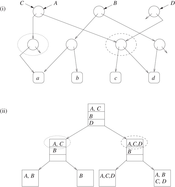
Figure 34.2The partition tree (ii) and its relation to the DAG created by the binary trie representation with shared subtrees.

34.4Extremal Sets and Subset Testing

This section deals with testing sets in $F$ $F$ for the subset containment relationship. We first survey a static version of this problem, and then consider a dynamisation.

34.4.1Static Extremal Sets

Here we assume that we are given a family $F$ $F$ of sets from a common universe as input. A set S is maximal in $F$ $F$ if there is no set $T \in F$ $T \in F$ such that S ⊂ T. A set S is minimal in $F$ $F$ if there is no set $T \in F$ $T \in F$ such that $S \supset T$ $S \supset T$ . The extremal sets problem is that of finding all the maximal (or all the minimal) sets in $F$ $F$ . A closely related problem is the computation of the complete subset graph, which represents all edges in the partial order induced among members of $F$ $F$ by the subset relation. Specifically, the complete subset graph is a directed graph whose vertices are the members of $F$ $F$ and there is an edge from x to y iff x ⊂ y. This is a problem that arises in a number of practical contexts, for example, it can be used to maximally simplify formulae in restricted conjunctive normal form [20].

This problem has been considered in a number of papers including [20–24]. We now summarize the results in these papers. As before, we let $k = | F |$ $k = | F |$ denote the size of the family, and $n = \sum_{S \in F} | S |$ $n = \sum_{S \in F} | S |$ be the total cardinality of all sets. A number of straightforward approaches can be found with a worst-case complexity of O(n2). It can be shown that the subset graph has Ω(n2/(log n)2) edges [21], which gives a lower bound for any algorithm that explicitly lists the complete subset graph. An aim, therefore, is to bridge the gap between these bounds; all results below are in the word RAM model.

Yellin and Jutla gave an algorithm that computes the subset graph using O(n2/ log n) dictionary operations. Using hashing, all dictionary operations take O(1) expected time, and we get an O(n2/ log n) expected running time. Using Willard’s q-fast tries [18], or the more complex data structure of Beame and Fich [19] gives running times of $O (n^{2} / \sqrt{\log n})$ $O (n^{2} / \sqrt{\log n})$ or O((n log log n)2/ log n) respectively. Pritchard [22] gave a simple algorithm that ran in O(n2/ log n) time. In [23] he re-analyzed an earlier algorithm [20] to show that this algorithm, too, ran in O(n2/ log n) time (the algorithm of [20,23] uses RAM operations less extensively and is a good candidate for porting to the pointer machine model). Finally, Pritchard [24] gave an algorithm that uses the bit-parallelism of the word RAM extensively to achieve an O(n log log n/(log n)2) running time.

All of the above are static problems—it is very natural to ask about the complexity of this problem when updates may change the sets in $F$ $F$ . Again, if one wishes explicitly to maintain the entire subset graph, it is easy to see that Ω(n) edges may change as the result of a single update. Take U = {1,…, u} and $F = {A, B_{2}, \dots, B_{u}}$ $F = {A, B_{2}, \dots, B_{u}}$ , where A = U and B_i = {1, i} for i = 2,…, u. The sum of the sizes of the sets in $F$ $F$ is 2u − 2, but deleting the element 1 from A removes all u − 1 edges from the complete subset graph. It is not very hard to come up with algorithms that can achieve an O(n) running time (see, e.g., [21]). To obtain a better complexity, therefore, we must consider algorithms that do not explicitly store this graph. One way of doing this is to consider the dynamic subset testing problem, defined as the problem of supporting the base repertoire (34.1) and the subset operation (34.5). Since the query subset(A, B) tests if there is an edge between A and B in the complete subset graph, this problem seems to be an appropriate dynamisation of the extremal sets problem, and it is dealt with in the next section.

34.4.2Dynamic Set Intersections and Subset Testing

Rather than consider the dynamic subset testing problem directly, we consider a related problem, the dynamic set intersection problem. In addition to the base repertoire (34.1) of actions above, we consider an enumerative version of the following:

$\begin{array}{ll} intersect (A, B) & Report the intersection of sets A and B . \end{array}$ $\begin{array}{ll} intersect (A, B) & Report the intersection of sets A and B . \end{array}$	(34.6)

Other variations could include returning the size of the intersection, or retrieving some values associated with the elements in the intersection. A unifying way to study these problems is as follows: we are given a set $M$ $M$ of information items that will be associated with elements of U, a function $I : U \to M$ $I : U \to M$ that associates values from M with keys in U. We assume that $M = (M, +, 0)$ $M = (M, +, 0)$ is a monoid. The query intersect(A, B) then returns $\sum_{x \in A \cap B} I (x)$ $\sum_{x \in A \cap B} I (x)$ , where the sum is taken with respect to +. It is easy to cast the intersection problem and its variants in this framework. The basic problem defined above can be obtained by letting $M = (2^{U}, \cup, {})$ $M = (2^{U}, \cup, {})$ and I(x) = {x} for all x, and the problem where one merely has to report the size of the intersection can be obtained by setting $M = (I N, +, 0)$ $M = (I N, +, 0)$ and I(x) = 1 for all x, where + here is normal (arithmetic) addition. Note that dynamic subset testing, defined in the previous section, easily reduces to the intersection problem: A ⊆ B iff |A| = |A ∩ B|.

We now survey the results in this area. It is useful to use the notation $\tilde{O} (f (n)) = \cup_{c = 0}^{\infty} O (f (n) \log^{c} n)$ $\tilde{O} (f (n)) = \cup_{c = 0}^{\infty} O (f (n) \log^{c} n)$ , which ignores polylogarithmic factors are ignored (a similar convention is used for the Ω notation, with inverse polylogarithmic factors being ignored).

For this problem, Yellin [25] gave an algorithm that processed a sequence of n insertions and deletions and q intersect operations in time $\tilde{O} (n \cdot n^{1 / k} + q n^{(1 - 1 / k)})$ $\tilde{O} (n \cdot n^{1 / k} + q n^{(1 - 1 / k)})$ time for any fixed k. The intuition behind this result is as follows. Take t = n^{1 − 1/k} and say that a set $S \in F$ $S \in F$ is large if |S| ≥ t and small otherwise. All sets are represented as dictionaries (allowing membership testing in logarithmic time). Intersections between two small sets, or between a small set and a large one, are handled by testing each element of one set for membership in the other. Clearly this takes $\tilde{O} (t)$ $\tilde{O} (t)$ time, and insertion into and deletion from a small set takes $\tilde{O} (1)$ $\tilde{O} (1)$ time. For every pair of large sets S, T, the algorithm keeps track of I(S ∩ T) explicitly, by storing the elements of S ∩ T in a balanced binary search tree, and storing at any internal node x the monoid sums of all the elements under x.^* Since there are at most n/t = n^1/k large sets, an insertion into, or a deletion from, a large set requires updating at most n^1/k of the pairwise intersections with other sets, and takes $\tilde{O} (n^{1 / k})$ $\tilde{O} (n^{1 / k})$ time. This proves the time bound, modulo some details such as dealing with changes in the value of t caused by changes in n and so on.

Dietz et al. [26] noticed that if one were to process a sequence of n updates and q queries, where n and q are known in advance, then the overall cost of Yellin’s algorithm for processing the sequence is minimized by taking $n^{1 / k} = min {n, \sqrt{q}}$ $n^{1 / k} = min {n, \sqrt{q}}$ , giving an overall time bound of $\tilde{O} (q + n \sqrt{q})$ $\tilde{O} (q + n \sqrt{q})$ . They gave an algorithm that achieves this bound even when n and q are not known in advance.

We now show that this bound is essentially tight in the arithmetic model, by giving a lower bound of $\tilde{Ω} (q + n \sqrt{q})$ $\tilde{Ω} (q + n \sqrt{q})$ . For simplicity, consider the problem where the elements in the intersection are to be reported, that is, take $M = (2^{U}, \cup, {})$ $M = (2^{U}, \cup, {})$ and I(x) = {x}. Starting from an empty family $F$ $F$ , we build it up by insertions so that the (sums of) sizes of the pairwise intersections of sets in $F$ $F$ are large, and query all possible intersections of the sets. If the answers to all the queries were to be obtained by adding (unioning) together singleton sets, then the lower bound would follow. Unfortunately, this is too simplistic: subsets obtained as temporary values during the computation of one answer may be re-used to answer another query. To get around this, we note that a subset that is used to compute the answer to several intersection queries must lie in the common intersection of all the sets involved, and construct $F$ $F$ so that the common intersection of any of a sufficiently large (yet small) number of sets in $F$ $F$ is small. This means that no large subset can be reused very often.

We assume that q ≤ n2 (otherwise the lower bound is trivial). Starting with an empty family, we perform a sequence of n = Θ(N) insert operations and q queries. We choose $U = {1, \dots, 2 N / \sqrt{q}}$ $U = {1, \dots, 2 N / \sqrt{q}}$ and $k = | F | = \sqrt{q}$ $k = | F | = \sqrt{q}$ ; we let m = |U| and let ℓ = c log N for some sufficiently large constant c > 0. We assume the existence of a family $F = {S_{1}, \dots, S_{k}}$ $F = {S_{1}, \dots, S_{k}}$ with the following properties:

a.|S_i ∩ S_j| = Ω(m) for all i, j with 1 ≤ i < j ≤ k.

b.for any pairwise distinct indices i1,…, i_ℓ, $| \cap_{j = 1}^{ℓ} S_{i_{j}} | < ℓ$ $| \cap_{j = 1}^{ℓ} S_{i_{j}} | < ℓ$ .

The existence of such a family is easily shown by a probabilistic argument (a collection of random sets of the appropriate size suffices). We now represent $F$ $F$ in the data structure by executing the appropriate insertions. Note that this requires at most km = N = Θ(n) update operations, since |S_i| ≤ m for all i. We then query the pairwise intersections of all the sets; there are (k 2) = Θ(q) queries in all.

Firstly, note that the sizes of all the output sets sum to Ω(mk2) by (a) above. The output to each query is conceptually obtained by a binary union tree in which each internal node combines the answers from its children; the external nodes represent singleton sets. Each node can be labeled with a set in the obvious way. Consider the entire forest; we wish to count the number of distinct nodes in the forest (that is, nodes labeled with distinct sets). Since each distinct set corresponds to at least one instruction that is not counted elsewhere, counting the number of distinct sets is a lower bound on the number of instructions executed.

We consider only nodes that correspond to sets of size ℓ or larger. Clearly, the number of such sets is Ω(mk2/ℓ). Furthermore, no such set can be used to answer more than (ℓ 2) different queries by (b). It follows that there are $Ω (m k^{2} / ℓ^{3}) = \tilde{Ω} (n \sqrt{q})$ $Ω (m k^{2} / ℓ^{3}) = \tilde{Ω} (n \sqrt{q})$ distinct sets, giving us a lower bound of this magnitude (as mentioned above, a lower bound of Ω(q) is trivial whenever $q = \tilde{Ω} (n \sqrt{q})$ $q = \tilde{Ω} (n \sqrt{q})$ ).

Dietz et al. also considered the relatively high memory usage of the above algorithms. For example, if q = Θ(n) then both Yellin’s algorithm and Dietz et al.’s algorithm use Ω(n^3/2) space. Dietz et al. also considered the complexity of the above problem when the algorithms were restricted to use s memory locations, where n ≤ s ≤ n2, and gave an algorithm that processed n operations (queries and updates) in $\tilde{O} (n / s^{1 / 3})$ $\tilde{O} (n / s^{1 / 3})$ time. Both the upper bound and the lower bound are more complex than those for the unlimited-memory case. We summarize with the main theorems of Dietz et al.:

Theorem 34.4

For the problem of maintaining a family of sets under create, insert, delete and intersect, we have the following results:

i.Any algorithm requires $\tilde{Ω} (q + n \sqrt{q})$ $\tilde{Ω} (q + n \sqrt{q})$ time to process a sequence of n updates and q queries in the arithmetic model of computation.

ii.Any intermixed sequence of n updates and q queries can be processed in $\tilde{O} (n \sqrt{q} + q)$ $\tilde{O} (n \sqrt{q} + q)$ time using $O (min {n \sqrt{q}, n^{2}})$ $O (min {n \sqrt{q}, n^{2}})$ space.

iii.There is a sequence of O(n) updates and queries that requires $\tilde{Ω} (n^{2} s^{- 1 / 3})$ $\tilde{Ω} (n^{2} s^{- 1 / 3})$ operations in the arithmetic model, if the algorithm is restricted to using s memory locations.

iv.Any intermixed sequence of O(n) updates and queries can be performed in $\tilde{O} (n^{2} / s^{1 / 3})$ $\tilde{O} (n^{2} / s^{1 / 3})$ time and O(s) space.

As mentioned above, the arithmetic model is a relatively weak one (making it easy to prove lower bounds), but all the algorithms that realise the upper bounds fit into this model. It would be interesting to prove similar lower bounds for stronger models or to design algorithms that improve upon the performance of the above in stronger models. Note also, that the lower bounds are for the intersection problem, not the problem that we originally considered, that of subset testing. Since we get back a boolean answer from a subset testing query, it does not fit into the arithmetic framework.

34.5The Disjoint Set Union-Find Problem

In this section we cover the best-studied set problem: the disjoint set union-find problem. The study of this problem and its variants has generated dozens of papers; indeed, it would not be unreasonable to devote an entire chapter to this problem alone. Fortunately, much of the work on this problem took place from the 1960s through to the early 1990s, and this work is surveyed in an excellent article by Galil and Italiano [27]. In this section, we summarise the main results prior to 1991 but focus on developments since then.

We begin with by formulating the problem in a recent, more general way [28], that fits better in our framework. We start with the base repertoire, but now require that insert(x, A) is only permitted if x ∉ B, for all sets $B \in F - {A}$ $B \in F - {A}$ . This ensures that all sets in $F$ $F$ are pairwise disjoint. We now add the following operations:

dunion(A, B, C) This sets $C \leftarrow A \cup B$ $C \leftarrow A \cup B$ , but destroys (removes from $F$ $F$ ) A and B.

find(x) For any $x \in \cup_{A \in F} A$ $x \in \cup_{A \in F} A$ , returns the name of the set that x is in.

This problem has a number of applications, beginning historically with the efficient implementation of EQUIVALENCE and COMMON statements in early FORTRAN compilers in the 1960s, and continues to find applications in diverse areas such as dynamic graph algorithms, meldable data structures and implementations of unification algorithms.

It is difficult to discuss the disjoint-set union-find problem without reference to Ackermann’s function, which is defined for integers i, n ≥ 0 as follows:

A (i, n) = {\begin{cases} 2 n & for i = 0, n \geq 0 \\ 1 & for i \geq 1, n = 0 \\ A (i - 1, A (i, n - 1)) & for i, n \geq 1 \end{cases}

$A (i, n) = {\begin{cases} 2 n & for i = 0, n \geq 0 \\ 1 & for i \geq 1, n = 0 \\ A (i - 1, A (i, n - 1)) & for i, n \geq 1 \end{cases}$

For a fixed i, the row inverse of Ackermann’s function, denoted by a(i, n), is defined as:

a (i, n) = min {j ∣ A (i, j) \geq n} .

$a (i, n) = min {j ∣ A (i, j) \geq n} .$

It can be verified that a(1, n) = Θ(log n) and a(2, n) = Θ( log^*n), where log^*n is the iterated logarithm function. The functional inverse of Ackermann’s function is defined for m, n ≥ 1 by:

α (m, n) = min {i \geq 1 ∣ A (i, 4 ⌈ m / n ⌉) \geq n}

$α (m, n) = min {i \geq 1 ∣ A (i, 4 ⌈ m / n ⌉) \geq n}$

Since $A (3, 4) = 2^{2^{\cdot^{\cdot^{\cdot^{2}}}}}} 65, 536 times$ $A (3, 4) = 2^{2^{\cdot^{\cdot^{\cdot^{2}}}}}} 65, 536 times$ , for all practical purposes, α(m, n) ≤ 3 whenever m, n ≥ 1. Indeed, if m grows sufficiently faster than n (e.g., m = Ω(n log^*n)) then α(m, n) is indeed a constant.

The union-find problem in the above formalisation was studied by [29], who gave the following results:

Theorem 34.5

i.An intermixed sequence of f find, m insert, m create, d ≤ m delete operations and at most m − 1 dunion operations takes O(m + (f + d)α(f + m, m)) time. The size of the data structure at any time during the sequence is proportional to the number of live items in it.

ii.For any parameter k > 1, an intermixed sequence of find, dunion, insert, create, and delete operations can be processed in the following worst-case time bounds: find and delete in O(log m/ log k) time, create and insert in O(1) time and dunion in O(k) time, where m is the current number of elements in the data structure.

In fact, [29] showed that this problem could be reduced to the classical union-find problem (see below). This reduction is such that the time bounds for find and dunion change only by a constant factor, but the time to delete an element x is the same as the time it takes to find the set containing x plus the time it takes to unite a singleton set with this set. The results follow by applying this result, respectively, to the classical union-find data structures given in Theorem 34.6(i) and Theorem 34.6(ii) (in fact they use a variant of the latter result due to Smid [30]).

An interesting variant of the above problem was considered by the same authors in [28]. They replaced the find operation with the seemingly simpler:

bfind(x, A) Return “true” if x ∈ A and “false” otherwise.

This “boolean” union-find problem was motivated by the problem of implementing meldable priority queues. Kaplan et al. showed that the lower bounds established for the classical union-find problem apply to this problem as well (see Theorem 34.7).

34.5.1The Classical Union-Find Problem and Variants

In the classical version of this problem, we have U = {1,…, m} and $F$ $F$ initially equals {{1},{2},…,{m}}; we assume that the name of the set {i} is simply i. The operation dunion is modified as follows:

dunion(A, B) This sets $A \leftarrow A \cup B$ $A \leftarrow A \cup B$ , but destroys (removes from $F$ $F$ ) B.

The operation find(x) operates as described above. We now mention the main upper bounds that are known for the classical version of the problem:

Theorem 34.6

A sequence of m − 1 dunion and f find operations can be processed as follows:

i.in O(m + fα(f + m, m)) time;

ii.for any parameter k > 1, each find takes O(log m/(log k + log log m)) worst-case time and each dunion takes O(k) worst-case time;

iii.the ith find operation takes O(α(i, m)) worst-case time, and the entire sequence takes O(m + fα(f + m, m)) time;

iv.for any parameter k > 0, the entire sequence takes O(ma(k, m) + kf) time;

v.for any parameter k > 1, dunion takes O(k) worst-case time, find takes t_q = O(log m/ log k) worst-case time, and the entire sequence takes time O((m + f)(α(m + f, m) + a(t_q, m)) time.

We begin by remarking that the bounds (i) and (ii) are in fact implied by Theorem 34.5, but are included here for completeness (see [27] for a more complete history). The upper bound of Theorem 34.5(i) is due to Tarjan [31] (with many interesting refinements due to [32]). Note that since α(f + m, m) is essentially constant, the running time is linear for all practical purposes. In (i), each dunion takes O(1) worst-case time, but a single find may take Ω(log m) time. Result (iii) allows us to process each find quickly, in essentially constant time, but an individual dunion could be quite slow and may in fact take Ω(m) time. The overall cost of the sequence remains as in (i), though. This was explicitly proved in [33], but the main ideas were already present in [34]. In (iv), the time for a dunion is traded off for find, and the overall running time remains essentially linear (at least for k ≥ 2) [35].

In either (i) or (iii), although the overall cost of the operation sequence is very low, an individual operation could take Ω(log m) or Ω(m) time respectively. If we wish to minimise the maximum cost of a single operation over the sequence, then choosing (say) $k = Θ (\sqrt{\log m})$ $k = Θ (\sqrt{\log m})$ in (ii), we get that no operation takes more than O(log m/ log log m) time. However, the cost of the entire sequence increases to Ω(f log m/ log log m). This result is due to [36].

In [37], the authors ask the question whether one can combine the best features of the results (i) (or (iii)) and (ii). Except possibly for a few extreme cases, this is achieved in [37, Theorem 11]. The result presented there has some technical restrictions (e.g., the algorithm needs to know the value of m in advance), but the authors claim that these are not essential.

We now come to lower bounds for this problem, which are either proved in the pointer machine model or the cell probe model. In general the cell probe model is more powerful (since there are no restrictions on the way that memory is accessed), but the lower bounds are proven assuming that all memory locations can store only numbers of O(log m) bits. By contrast, the pointer machine model does not place any restrictions on the size of the numbers that can be stored at each node. In the pointer machine model, however, the algorithm is required to maintain the name of each set in distinct nodes, and an operation such as find(x) must traverse the graph of nodes from the node for x to the node that contains the name of the set that x is in. Lower bounds for the pointer machine model sometimes make the following separability assumption [3]:

At any time during the computation, the contents of the memory can be partitioned into collections of records such that each collection corresponds to a currently existing set, and no record in one collection contains a pointer to a record in another collection.

We now give some of the known lower bounds:

Theorem 34.7

i.Any algorithm that processes a sequence of m − 1 dunion and f find operations must take Ω(m + fα(f + m, m)) steps on either the pointer machine model or the cell probe model with a word size of O(log m) bits.

ii.Any algorithm that processes a sequence of m − 1 dunion and f find operations must take Ω(log m/ log log m) steps for some operation, on either the separable pointer machine model or the cell probe model with a word size of O(log m) bits.

The lower bound (i) for the pointer machine model is due to [38]; this generalizes an earlier lower bound for separable pointer machine algorithms due to [3] (see also the result due to [39]). The lower bound (ii) is due to [36], while both cell probe lower bounds are due to [40]. Additional lower bounds may be found in [37].

We refer the reader to [27] for variations of the classical union-find problem, including union-find with backtracking and persistent union-find (for the latter, see also [41,42]). Another important variant, which has a similar complexity to that of the union-find problem, is the split-find problem. Here we are given an ordered universe U and start with $F$ $F$ containing a single set which contains all of U. We perform an intermixed series of operations $S, T \leftarrow split (S, x)$ $S, T \leftarrow split (S, x)$ for some x ∈ S, which removes from S all elements > x and places them in a new set T, and find(x), which as before returns the name of the set containing x. Upper and lower bounds of the form given in Theorems 34.6(i) or 34.7(i) have been proven by [33,34, 38]. Finally, we mention the very interesting Union-copy problem studied in [43]. In addition to the classical union-find operations, they support an additional operation copy, which takes one set as its argument, and adds an exact copy of it to $F$ $F$ . Although it is obviously no longer true that all sets in $F$ $F$ are disjoint, they require that two sets that are to be united must be disjoint. In addition, they want the data structure to support dual operations, in the sense that the roles of sets and elements are reversed. For example, the operation element-union(x, y) takes two elements x and y that do not both belong to any set in $F$ $F$ , and turns them into a single element that is member of all the sets to which x or y previously belonged. Duals of copy and find are also supported. They show applications of this data structure to the (geometric) dynamic segment tree data structure.

34.6Partition Maintenance Algorithms

A partition P of a given universe U = {1,2,…, m} is a collection of #P disjoint subsets (parts), P⁽¹⁾, P⁽²⁾,…, P^(#P), of U such that ∪_iP_i = U. A case of special interest is that of bipartitions, which is a partition with two parts. A partition P is an equivalence relation on U, which we denote as ≡ _P. Given two partitions P and Q, the induced partition of P and Q is the partition that represents the equivalence relation x ≡ y⇔((x ≡_P y)∨(x≡_Qy)) (in words, two elements belong to the same part of the induced partition iff they belong to the same part in both P and Q). The problem we consider is the following. Given a collection $F$ $F$ of partitions (initially empty), to support the following operations:

$\begin{array}{ll} report (F) & Report the partition induced by the members of F . \\ insert (P) & Add partition P to F . \\ delete (P) & Remove partition P from F . \end{array}}$ $\begin{array}{ll} report (F) & Report the partition induced by the members of F . \\ insert (P) & Add partition P to F . \\ delete (P) & Remove partition P from F . \end{array}}$	(34.7)

We assume here that each new partition P is given by an array A[1..m] containing integers from 0 to #P − 1. Other operations include asking if two elements belong to the same partition of the global induced partition, reporting the set of elements that belong to the same part of the global induced partition, or, for any two elements, reporting the number of partitions in which these two elements are in different parts.

As noted by Bender et al. [44] and Calinescu [45], this problem has a number of applications. The general issue is supporting a classification system that attempts to categorize objects based on a number of tests, where each test realizes a partition of the objects (a bipartition, for instance, could model the outcome of a boolean test). The above data structure would be useful in the pre-processing phase of such a classification system, where, for example, an algorithm may repeatedly insert and delete partitions (tests) until it finds a small set of tests that distinguish all items of the universe. Examples in optical character recognition (OCR) and VLSI are given by the above authors.

We now discuss some solutions to these problems. The model used is the word RAM model with word size Θ(log n), where we take $k = | F |$ $k = | F |$ and n = km. We first consider the case of general partitions, and then that of bipartitions. A simple data structure for general partitions was given by Bender et al. [44], and resembles the partition tree of Section 34.3. A key fact they use is (apply radix sorting on triples of the form 〈P[i], Q[i], i〉):

Proposition 34.1

Given two partitions P and Q of U = {1,…, m} we can calculate the induced partition of P and Q in O(m) time.

This immediately implies that we can maintain the induced partition of $F$ $F$ under inserts alone in O(m) time and also support report in O(m) time—we simply maintain the global induced partition and update it with each insert. deletes are not so easy, however.

We place the partitions at the leaves of a full binary tree with k leaves. At each internal node v of this binary tree we store the partition induced by all the partitions descended from v. Clearly, the root contains the global induced partition. Inserting a partition P involves replacing a leaf containing a partition Q by an internal node that has P and Q as children, and updating the partitions stored at this internal node and all its ancestors. Deleting a partition involves deleting the appropriate leaf, and maintaining fullness by possibly swapping a “rightmost” leaf with the deleted leaf. In either case, we update partitions from at most two leaves up to the root. This gives a data structure that supports insert and delete in O(m log k) time and report in O(m) time. The space used is O(mn) words of memory.

The time for insert can be improved to amortised O(m), while leaving the time complexity of all other operations the same. The idea is to group all partitions into disjoint groups of t = ⌈ log k⌉ each, leaving perhaps one incomplete group of size smaller than t. For each group we store its induced partition, and also store the induced partitions of all groups, except the incomplete group, at the leaves of a tree T (which may now have O(k/ log k) leaves) as before. In addition, we explicitly store the global induced partition G.

When performing insert(P) we add P to the incomplete group and in O(m) time, update the global partition G. If the incomplete group reaches size t, in addition, we calculate the group’s induced partition in O(mt) = O(m log k) time and insert this induced partition into T, also taking O(m log k) time, and start a new empty incomplete group. Deleting a partition P is done as follows. We delete P from its group. If P is in the incomplete group we recompute the G in O(mt) time. If P’s group is stored in T, we recompute the new partition induced by P’s group in O(mt) time and update T in O(m log k) time (if P is the last remaining partition in its group we delete the corresponding leaf, as before). We then recompute G in O(mt) = O(m log k) time as well. Note that the amortised cost of an insertion is now O(m), since we spend O(m log k) time every log k insertions. Finally, Bender et al. note that a signature-based scheme gives a Monte-Carlo method that performs all operations in O(m) time, but has a small chance of outputting an incorrect result (the algorithm runs correctly with probability 1 − O(m^−c) on all inputs).

We now consider the important special case of bi-partitions, and give a sketch of Calinescu’s [45] algorithm for solving this problem in optimal amortised time. Again letting $k = | F |$ $k = | F |$ , one can associate a k-bit binary string σ_x with each $x \in U = {1, \dots, m}$ $x \in U = {1, \dots, m}$ , which specifies in which part of each of the k partitions x lies. Let π denote a permutation such that σ_{π⁻¹ (i)} ≤ σ_{π⁻¹(i + 1)}, for i = 1,…, m − 1; that is, π represents a sorted order on the (multi-set) of strings {σ_x|x ∈ U}. Furthermore, let lcp_i denote the most significant position where σ_π⁻¹(i) and σ_{π⁻¹(i + 1)} differ, for i = 1,…, m − 1 (lcp_i = k + 1 if σ_π⁻¹(i) = σ_{π⁻¹(i + 1)}). We can now clearly support report in O(m) time, as elements in the same part of the global induced partition will be consecutive in sorted order, and the lcp values allow us to determine the boundaries of parts of the global induced partition without inspecting the strings. An insert of a partition is also easily supported, as only local re-arrangements of elements lying within the same part of the previous global induced partition are required.

Deleting a partition is a little harder, and requires a few observations. Suppose that we delete the partition that gives the tth most significant bit of σ1,…, σ_m. Suppose that for two indices i, j, j > i, lcp_i < t and lcp_j < t, but all lcp’s in between are at least t. Then we can conclude that the strings in positions 1 to i − 1 of the sorted order continue to appear in (possibly a different order in) positions 1 to i − 1 after the deletion of this partition, and likewise the strings in positions j + 1 to m also do not “move” except internally. Let Σ denote the strings that appear in positions i through j in sorted order, that is, Σ = {σ_l | l ∈ {π⁻¹(i), π⁻¹(i + 1), …, π⁻¹(j)}}. We now show how to sort Σ, and repeated application of this procedure suffices to re-sort the array. Note that all the strings in Σ that have 0 in the tth position maintain their relative order after the deletion, and likewise those strings with 1 in the tth position. Thus, re-sorting Σ is simply a matter of merging these two sets of strings. At a high level, the merging procedure proceeds like the (standard, trivial) algorithm. However, a naive approach would require Θ(k) time per comparison, which is excessive. Instead, we note that at each step of the merging, the next candidate can either be determined in O(1) time (when the relative order of the two candidates is implicit from the lcp data) or a number, c, of comparisons need to be made. However, if c comparisons are made, then there is at least one lcp value in the new array that is c more than its counterpart in the old array. Since lcp values are bounded by O(k), no string will be involved in more than O(k) comparisons during its lifetime, and the cost of these comparisons can be charged to the insertions of the partitions. This intuition can be formalized by a potential function argument to show that the amortised cost of a deletion is indeed O(n), thus giving an optimal (amortised) algorithm for this problem.

34.7Conclusions

We have presented a number of algorithms and data structures for supporting (largely) basic set-theoretic operations. Aside from the union-find problem, which has been extensively studied, relatively little research has been done into these problems. For instance, even the most basic problem, that of finding a general-purpose data structure that supports basic set operations, is not yet satisfactorily solved. The problem becomes more acute if one is concerned about the space usage of the data structures—for example, it is not known whether one can solve set equality testing efficiently in linear space.

Due to the proliferation of unstructured data, set operations are increasingly important. For instance, many search engines return a set of documents that match a given boolean keyword query by means of set operations on the sets of documents that contain each of the keywords in the query. The characteristics of this kind of application also suggest directions for research. For example, given the large data-sets that could be involved, it is a little surprising that work on external-memory algorithms for these problems is somewhat limited. Another issue is that these sets usually have patterns (e.g., the number of sets that contain a given keyword may satisfy a power law; certain sets of keywords may be more likely to be queried together etc.), which should be exploited by efficient algorithms.

With the latter motivation in mind, Demaine et al. [46] have considered the adaptive complexity of these problems. They assume that they are given a collection of sorted lists that comprise the sets, and need to compute unions, intersections and differences of these sets. If one is only interested in worst-case complexity (across all instances) then this problem is uninteresting (it essentially boils down to merging). However, some instances can be harder than others: for instance, computing the intersection of two sets when all elements in one set are smaller than the other is much easier than for sets that interleave substantially. Building on this idea, they develop a notion of the complexity of a given instance of a problem and develop algorithms that, for each particular instance, are efficient with respect to the difficulty of that instance.

References

1.A. N. Kolmogorov. On the notion of algorithm. Uspekhi Matematicheskikh Nauk, 8, 1953, pp. 175–176.

2.A. Schönage. Storage modification machines. SIAM Journal on Computing, 9, 1980, pp. 490–508.

3.R. E. Tarjan. A class of algorithms which require non linear time to maintain disjoint sets. Journal of Computer and System Sciences, 18, 1979, pp. 110–127.

4.A. V. Aho, J. E. Hopcroft and J. D. Ullman. The Design and Analysis of Computer Algorithms. Addison Wesley, 1974.

5.T. Hagerup. Sorting and searching on the word RAM. In Proc. 15th Symposium on Theoretical Aspects of Computer Science (STACS 1998), Lecture Notes in Computer Science, Springer-Verlag, Berlin, vol. 1373, pp. 366–398, 1998.

6.M. L. Fredman. A lower bound on the complexity of orthogonal range queries. Journal of the ACM, 28, 1981, pp. 696–705.

7.A. C. Yao. On the complexity of maintaining partial sums. SIAM Journal on Computing, 14, 1985, pp. 277–288.

8.K. Mehlhorn. Data Structures and Algorithms, Vol. III: Multi-dimensional Searching and Computational Geometry. Springer-Verlag, Berlin, 1984.

9.W. Pugh. Incremental computation and the incremental evaluation of function programs. PhD thesis, Cornell University, 1989.

10.W. Pugh and T. Teitelbaum. Incremental computation via function caching. In Conference Record of the 16th Annual ACM Symposium on Principles of Programming Languages, ACM, pp. 315–328, 1989.

11.D. E. Knuth. The Art of Computer Programming, vol. 3, 2nd Ed. Addison Wesley, 1998.

12.R. Seidel and C. Aragon. Randomized search trees. Algorithmica, 16, 1996, pp. 464–497.

13.R. Sundar and R. E. Tarjan. Unique binary-search-tree representations and equality testing of sets and sequences. SIAM Journal on Computing, 23, 1994, pp. 24–44.

14.A. Andersson and T. Ottmann. New tight bounds on uniquely represented dictionaries. SIAM Journal on Computing, 24, 1995, pp. 1091–1101.

15.D. M. Yellin. Representing sets with constant time equality testing. Journal of Algorithms, 13, 1992, pp. 353–373.

16.T. W. Lam and K. H. Lee. An improved scheme for set equality testing and updating. Theoretical Computer Science, 201, 1998, pp. 85–97.

17.M. H. Overmars. The Design of Dynamic Data Structures, vol. 156. Lecture Notes in Computer Science. Springer-Verlag, Berlin, 1983.

18.D. E. Willard. New trie data structures which support very fast search operations.

19.P. Beame and F. E. Fich. Optimal bounds for the predecessor problem and related problems. Journal of Computer and System Sciences, 65, 2002, pp. 38–72.

20.P. Pritchard. Opportunistic algorithms for eliminating supersets. Acta Informatica, 28, 1991, pp. 733–754.

21.D. M. Yellin and C. S. Jutla. Finding extremal sets in less than quadratic time. Information Processing Letters, 48, 1993, pp. 29–34.

22.P. Pritchard. A simple sub-quadratic algorithm for computing the subset partial order. Information Processing Letters, 56, 1995, pp. 337–341.

23.P. Pritchard. An old sub-quadratic algorithm for finding extremal sets. Information Processing Letters, 62, 1997, pp. 329–334.

24.P. Pritchard. A fast bit-parallel algorithm for computing the subset partial order. Algorithmica, 24, 1999, pp. 76–86.

25.D. M. Yellin. An algorithm for dynamic subset and intersection testing. Theoretical Computer Science, 129, 1994, pp. 397–406.

26.P. F. Dietz, K. Mehlhorn, R. Raman, and C. Uhrig. Lower bounds for set intersection queries. Algorithmica, 14, 1995, pp. 154–168.

27.Z. Galil and G. F. Italiano. Data structures and algorithms for disjoint set union problems. ACM Computing Surveys, 23, 1991, pp. 319–344.

28.H. Kaplan, N. Shafrir, and R. E. Tarjan. Meldable heaps and boolean union-find. In Proc. 34th Annual ACM Symposium on Theory of Computing, ACM, pp. 573–582, 2002.

29.H. Kaplan, N. Shafrir, and R. E. Tarjan. Union-find with deletions. In Proc. 13th Annual ACM-SIAM Symposium on Discrete Algorithms, ACM/SIAM, pp. 19–28, 2002.

30.M. Smid. A data structure for the union-find problem having good single-operation complexity. In Algorithms Review, Newsletter of the ESPRIT II Basic Research Action program project no. 3075, 1, ALCOM, 1990.

31.R. E. Tarjan. Efficiency of a good but not linear set union algorithm. Journal of the ACM, 22, 1975, pp. 215–225.

32.R. E. Tarjan and J. van Leeuwen. Worst-case analysis of set union algorithms. Journal of the ACM, 31, 1984, pp. 245–281.

33.J. A. La Poutré. New techniques for the union-find problem. In Proc. 1st Annual ACM-SIAM Symposium on Discrete Algorithms, ACM/SIAM, pp. 54–63, 1990.

34.H. N. Gabow. A scaling algorithm for weighted matching on general graphs. In Proc. 26th Annual Symposium on Foundations of Computer Science, IEEE Computer Society, pp. 90–100, 1985.

35.A. M. Ben-Amram and Z. Galil. On data structure tradeoffs and an application to union-find. Electronic Colloquium on Computational Complexity, Technical Report TR95-062, 1995.

36.N. Blum. The single-operation worst case.

37.S. Alstrup, A. M. Ben-Amram, and T. Rauhe. Worst-case and amortised optimality in union-find (extended abstract). In Proc. 31st Annual Symposium on Theory of Computing, ACM, pp. 499–506, 1999.

38.J. A. La Poutré. Lower bounds for the union-find and the split-find problem on pointer machines. Journal of Computer and System Sciences, 52, 1996, pp. 87–99.

39.L. Banachowsky. A complement to Tarjan’s result about the lower bound on the complexity of the set union problem. Information Processing Letters, 11, 1980, pp. 59–65.

40.M. L. Fredman and M. Saks. The cell probe complexity of dynamic data structures. In Proc. 21st Annual ACM Symposium on Theory of Computing, ACM, pp. 345–354, 1989.

41.P. F. Dietz and R. Raman. Persistence, amortisation and randomisation. In Proc. 2nd Annual ACM-SIAM Symposium on Discrete Algorithms, ACM/SIAM, pp. 77–87, 1991.

42.P. F. Dietz and R. Raman. Persistence, randomization and parallelization: On some combinatorial games and their applications (Abstract). In Proc. 3rd Workshop on Algorithms and Data Structures, Lecture Notes in Computer Science, Springer-Verlag, vol. 709, pp. 289–301, 1993.

43.M. J. van Kreveld, and M. H. Overmars. Union-copy data structures and dynamic segment trees. Journal of the ACM, 40, 1993, pp. 635–652.

44.M. A. Bender, S. Sethia, and S. Skiena. Data structures for maintaining set partitions. Manuscript, 2004. Preliminary version. In Proc. 7th Scandinavian Workshop on Algorithm Theory, Lecture Notes in Computer Science, Springer-Verlag, Berlin, vol.1851, pp. 83–96, 2000.

45.G. Calinescu. A note on data structures for maintaining partitions. Manuscript, 2003.

46.E. D. Demaine, A. López-Ortiz, and J. I. Munro. Adaptive set intersections, unions and differences. In Proc. 12th Annual ACM-SIAM Symposium on Discrete Algorithms, ACM/SIAM, pp. 743–752, 2001.

^*This chapter has been reprinted from first edition of this Handbook, without any content updates.

^*To some readers, the idea that the wordsize of a machine can change as we update the data structure may appear a little strange, but it is merely a formal device to ensure reasonable usage.

^*The operation for creating a new node is called a Cons.

^*If the monoid is $M = (2^{U}, \cup, {})$ $M = (2^{U}, \cup, {})$ , we do not store the monoid sum explicitly, but instead take the monoid sum at an internal node to be implicitly represented by the subtree rooted at it.

..................Content has been hidden....................

You can't read the all page of ebook, please click here login for view all page.

Table of Contents for 34. Data Structures for Sets

Create new playlist

Sign In

Sign Up

Table of Contents for
34. Data Structures for Sets