
Chris Okasaki
United States Military Academy
Data Structures in Functional Languages•Functional Data Structures in Mainstream Languages
41.3Binary Search Trees: Path Copying
41.4Skew Heaps: Amortization and Lazy Evaluation
A functional data structure is a data structure that is suitable for implementation in a functional programming language, or for coding in an ordinary language like C or Java using a functional style. Functional data structures are closely related to persistent data structures and immutable data structures—in fact, the three terms are often used interchangeably. Howevber, there are subtle differences.
•The term persistent data structures refers to the general class of data structures in which an update does not destroy the previous version of the data structure, but rather creates a new version that co-exists with the previous version. See Chapter 33 for more details about persistent data structures.
•The term immutable data structures emphasizes a particular implementation technique for achieving persistence, in which memory devoted to a particular version of the data structure, once initialized, is never altered.
•The term functional data structures emphasizes the language or coding style in which persistent data structures are implemented. Functional data structures are always immutable, except in a technical sense discussed in Section 41.4.
In this chapter, we will discuss the main issues surrounding the implementation of data structures in functional languages, and illustrate these issues with several extended examples. We will also show how to adapt functional data structures to a mainstream language such as Java, for use when a persistent data structure is required. Readers wishing more details about functional data structures should consult Okasaki [1].
41.1.1Data Structures in Functional Languages
Functional programming languages differ in several important ways from ordinary programming languages like C or Java, and these differences can sometimes have a large effect on how data structures are implemented. The main differences (at least from the perspective of data structures) are immutability, recursion, garbage collection, and pattern matching.
41.1.1.1Immutability
In functional languages, variables and records cannot be modified, or mutated, once they have been created.† Many textbook data structures depend critically on the ability to mutate variables and records via assignments. Such data structures can be difficult to adapt to a functional setting.
41.1.1.2Recursion
Functional languages frequently do not support looping constructs, such as for-loops or while-loops, because such loops depend on being able to mutate the loop control variable. Functional programmers use recursion instead.*
41.1.1.3Garbage Collection
Functional languages almost always depend on automatic garbage collection. Because objects are immutable in functional languages, they are shared much more widely than in ordinary languages, which makes the task of deciding when to deallocate an object very complicated. In functional languages, programmers ignore deallocation issues and allow the garbage collector to deallocate objects when it is safe to do so.
41.1.1.4Pattern Matching
Pattern matching is a method of defining functions by cases that are essentially textual analogues of the kinds of pictures data-structure designers often draw. Pattern matching is not supported by all functional languages, but, when available, it allows many data structures to be coded very concisely and elegantly.
41.1.2Functional Data Structures in Mainstream Languages
Even if you are programming in a mainstream language, such as C or Java, you may find it convenient to use a functional data structure. Functional data structures offer three main advantages in such a setting: fewer bugs, increased sharing, and decreased synchronization.
41.1.2.1Fewer Bugs
A very common kind of bug arises when you observe a data structure in a certain state and shortly thereafter perform some action that assumes the data structure is still in that same state. Frequently, however, something has happened in the meantime to alter the state of the data structure, so that the action is no longer valid. Because functional data structures are immutable, such alterations simply cannot occur. If someone tries to change the data structure, they may produce a new version of it, but they will in no way effect the version that you are using.
41.1.2.2Increased Sharing
Precisely to avoid the kinds of bugs described above, programmers in mainstream languages are careful to limit access to their internal data structures. When sharing is unavoidable, programmers will often clone their data structures and share the clones rather than granting access to their own internal copies. In contrast, functional data structures can be shared safely without cloning. (Actually, functional data structures typically perform a substantial amount of cloning internally, but this cloning is of individual nodes rather than entire data structures.)
41.1.2.3Decreased Synchronization
Again, precisely to avoid the kinds of bugs described above, programmers in concurrent settings are careful to synchronize access to their data structures, so that only a single thread can access the data structure at a time. On the other hand, because functional data structures are immutable, they can often be used with little or no synchronization. Even simultaneous writes are not a problem, because each writer thread will get a new version of the data structure that reflects only its own updates. (This assumes, of course, an application where participants do not necessarily want to see changes made by all other participants.)
Stacks (see Chapter 2) represented as singly-linked lists are perhaps the simplest of all data structures to make persistent. We begin by describing functional stacks supporting four main primitives:
•empty: a constant representing the empty stack.
•push(x,s): push the element x onto the stack s and return the new stack.
•top(s): return the top element of s.
•pop(s): remove the top element of s and return the new stack.
We can see right away several differences between this interface and the interface for ordinary stacks. First, for ordinary stacks, push and pop would implicitly change the existing stack s rather than returning a new stack. However, the hallmark of functional data structures is that update operations return a new version of the data structure rather than modifying the old version. Second, ordinary stacks would support a function or constructor to create a fresh, new stack, rather than offering a single constant to represent all empty stacks. This highlights the increased sharing possible with functional data structures. Because pushing an element onto the empty stack will not change the empty stack, different parts of the program can use the same empty stack without interfering with each other.
Figure 41.1 shows an implementation of stacks in Haskell [2], a popular functional programming language. Figure 41.2 shows a similar implementation in Java. Like all code fragments in this chapter, these implementations are intended only to illustrate the relevant concepts and are not intended to be industrial strength. In particular, all error handling has been omitted. For example, the top and pop operations should check whether the stack is empty. Furthermore, programming conventions in Haskell and Java have been ignored where they would make the code harder for non-fluent readers to understand. For example, the Haskell code makes no use of currying, and the Java code makes no attempt to be object-oriented.
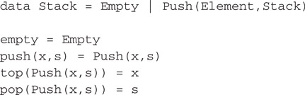
Figure 41.1Stacks in Haskell.
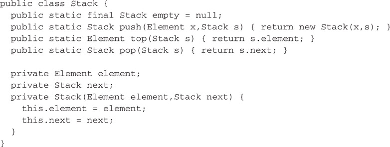
Figure 41.2Stacks in Java.
The Haskell code illustrates a simple use of pattern matching. The declaration
data Stack = Empty | Push(Element,Stack)
states that stacks have two possible shapes, Empty or Push, and that a stack with the Push shape has two fields, an element and another stack. The tags Empty and Push are called constructors. Later function declarations can match against these constructors. For example, the declaration
top(Push(x,s)) = x
says that when top is called on a stack with the Push shape, it returns the contents of the first field. If desired, more clauses can be added to deal with other shapes. For example, a second clause could be added to the definition of top to handle the error case:
top(Push(x,s)) = xtop(Empty) = ...signal an error...
How do these implementations achieve persistence? First, consider the push operation. Calling push creates a new node containing the new element and a pointer to the old top of stack, but it in no way alters the old stack. For example, if the old stack s contains the numbers 3, 2, 1 and we push 4, then the new stack s′ contains the numbers 4, 3, 2, 1. Figure 41.3 illustrates the relationship between s and s′. Notice how the nodes containing 3, 2, and 1 are shared between both stacks. Because of this sharing, it is crucial that the nodes are immutable. Consider what would happen if nodes could be changed. If we were to change the 3 to a 5, for example, perhaps by calling an operation to update the top element of s, that change would affect not only s (which would now contain 5, 2, 1) but also s′ (which would now contain 4, 5, 2, 1). Such unintended consequences would make sharing impossible.
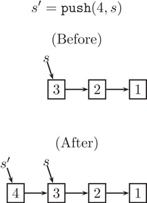
Figure 41.3The push operation.
Next, consider the pop operation, which simply returns the next pointer of the current node without changing the current node in any way. For example, Figure 41.4 illustrates the result of popping the stack s′ to get the stack s′′ (which shares its entire representation with the original stack s). Notice that, after popping s′, the node containing 4 may or may not be garbage. It depends on whether any part of the program is still using the s′ stack. If not, then automatic garbage collection will eventually deallocate that node.
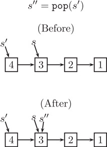
Figure 41.4The pop operation.
41.3Binary Search Trees: Path Copying
Stacks are unusual in that there is never a need to update an existing node. However, for most data structures, there is such a need. For example, consider inserting an element into a binary search tree (see Chapter 3). At the very least, we need to update the new node’s parent to point to the new node. But how can we do this if nodes are immutable? The solution is a technique called path copying. To update an existing node, we copy the node and make the necessary changes in the copy. However, we then have to update the existing node’s parent in a similar fashion to point to the copy. In this way, changes propagate all the way from the site of the update to the root, and we end up copying that entire path. That may seem like a lot of copying, but notice that all nodes not on that path are shared between the old and new versions.
To see how path copying works in practice, consider a simple implementation of integer sets as unbalanced binary search trees. Figure 41.5 shows an implementation in Haskell and Figure 41.6 shows the same implementation in Java.
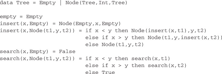
Figure 41.5Binary search trees in Haskell.
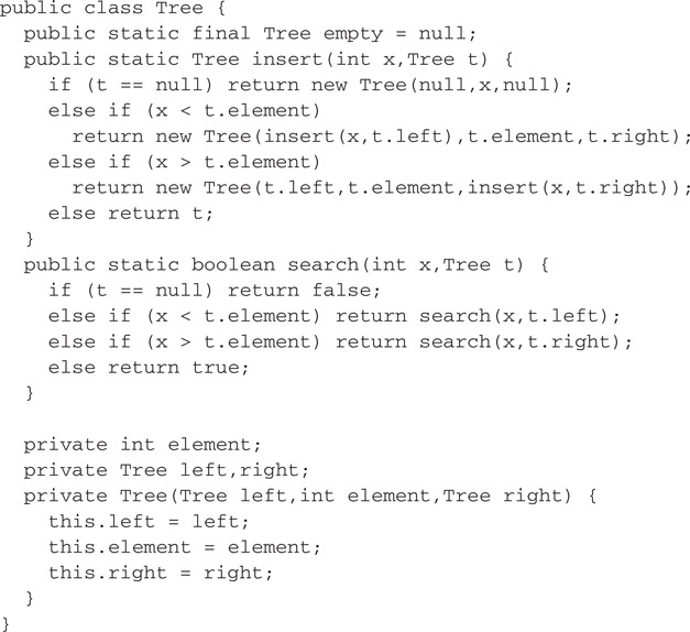
Figure 41.6Binary search trees in Java.
The key to understanding path copying lies in the insert operation. Consider the case where the element being inserted is larger than the element at the current node. In the Java implementation, this case executes the code
return new Tree(t.left,t.element,insert(x,t.right));
First, insert calls itself recursively on the right subtree, returning a pointer to the new right subtree. It then allocates a new tree node, copying the left and element fields from the old node, and installing the new pointer in the right field. Finally, it returns a pointer to the new node. This process continues until it terminates at the root. Figure 41.7 illustrates a sample insertion. Notice how the parts of the tree not on the path from the root to the site of the update are shared between the old and new trees.
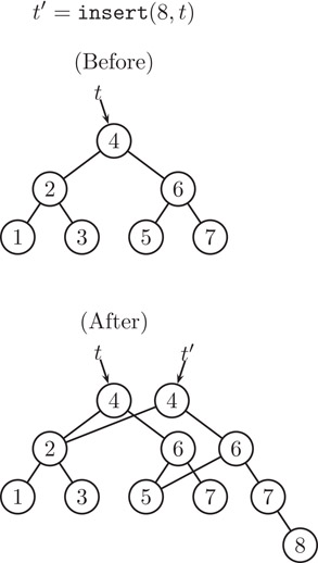
Figure 41.7The insert operation.
This functional implementation of binary search trees has exactly the same time complexity as an ordinary non-persistent implementation. The running time of insert is still proportional to the length of the search path. Of course, the functional implementation allocates more space, but even that issue is not clear cut. If the old tree is no longer needed, then the just-copied nodes can immediately be garbage collected, leaving a net space increase of one node—exactly the same space required by a non-persistent implementation. On the other hand, if the old tree is still needed, then the just-copied nodes cannot be garbage collected, but in that case we are actively taking advantage of functionality not supported by ordinary binary search trees.
Of course, the binary search trees described above suffer from the same limitations as ordinary unbalanced binary search trees, namely a linear time complexity in the worst case. Whether the implementation is functional or not as no effect in this regard. However, we can easily apply the ideas of path copying to most kinds of balanced binary search trees (see Chapter 11), such as AVL trees [3,4], red-black trees [5], 2-3 trees [6], and weight-balanced trees [7]. Such a functional implementation retains the logarithmic time complexity of the underlying design, but makes it persistent.
Path copying is sufficient for implementing many tree-based data structures besides binary search trees, including binomial queues [8,9] (Chapter 7), leftist heaps [1,10] (Chapter 5), Patricia tries [11] (Chapter 29), and many others.
41.4Skew Heaps: Amortization and Lazy Evaluation
Next, we turn to priority queues, or heaps, supporting the following primitives:
•empty: a constant representing the empty heap.
•insert(x,h): insert the element x into the heap h and return the new heap.
•findMin(h): return the minimum element of h.
•deleteMin(h): delete the minimum element of h and return the new heap.
•merge(h1,h2): combine the heaps h1 and h2 into a single heap and return the new heap.
Many of the standard heap data structures can easily be adapted to a functional setting, including binomial queues [8,9] and leftist heaps [1,10]. In this section, we describe a simple, yet interesting, design known as skew heaps [12]. (Non-persistent skew heaps are described in detail in Chapter 6.)
A skew heap is a heap-ordered binary tree. Each node contains a single element, and the nodes are ordered such that the element at each node is no larger than the elements at the node’s children. Because of this ordering, the minimum element in a tree is always at the root. Therefore, the findMin operation simply returns the element at the root. The insert and deleteMin operations are defined in terms of merge: insert creates a new node and merges it with the existing heap, and deleteMin discards the root and merges its children.
The interesting operation is merge. Assuming both heaps are non-empty, merge compares their roots. The smaller root (that is, the root with the smaller element) becomes the new overall root and its children are swapped. Then the larger root is merged with the new left child of the smaller root (which used to be the right child). The net effect of a merge is to interleave the rightmost paths of the two trees in sorted order, swapping the children of nodes along the way. This process is illustrated in Figure 41.8. Notice how the nodes on the rightmost paths of the arguments end up on the leftmost path of the result. A Haskell implementation of skew heaps incorporating path copying is shown in Figure 41.9. A naive Java implementation is shown in Figure 41.10.
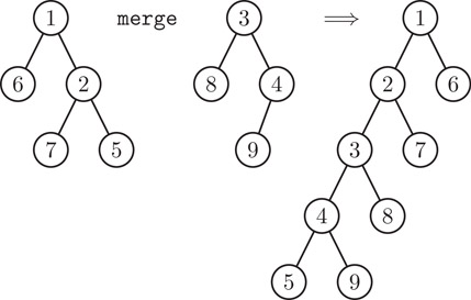
Figure 41.8Merging two skew heaps.
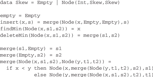
Figure 41.9Skew heaps in Haskell.
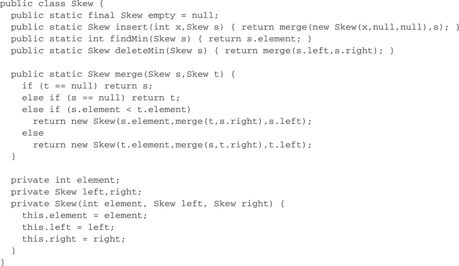
Figure 41.10First attempt at skew heaps in Java
Skew heaps are not balanced, and individual operations can take linear time in the worst case. For example, Figure 41.11 shows an unbalanced shew heap generated by inserting the elements
5, 6, 4, 6, 3, 6, 2, 6, 1, 6
into an initially empty heap. Inserting a new element such as 7 into this unbalanced skew heap would take linear time. However, in spite of the fact that any one operation can be inefficient, the way that children are regularly swapped keeps the operations efficient in the amortized sense—insert, deleteMin, and merge run in logarithmic amortized time [12].
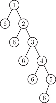
Figure 41.11An unbalanced skew heap.
Or, at least, those would be the bounds for non-persistent skew heaps. When we analyze skew heaps in a persistent setting, we receive a nasty shock. Making an amortized data structure such as skew heaps persistent using path copying breaks its amortized bounds! In the case of skew heaps, naively incorporating path copying causes the logarithmic amortized bounds to degrade to the linear worst-case bounds.
Consider, for example, the unbalanced skew heap s in Figure 41.11, for which insert takes linear time for large elements. The result of the insert is a new skew heap s′. Performing another insert on s′ would actually be quite efficient, but because these structures are persistent, we are free to ignore s′ and perform the next insert on the old skew heap s instead. This insert again takes linear time. We can continue performing operations on the old skew heap as often as we want. The average cost per operation over a sequence of such operations is linear, which means that the amortized cost per operation is now linear, rather than logarithmic. Simple experiments on the Java implementation from Figure 41.10 confirm this analysis.
However, if we repeat those experiments on the Haskell implementation from Figure 41.9, we do not observe linear behavior. Instead, the operations appear to retain their logarithmic amortized bounds, even under persistent usage. This pleasant result is a consequence of a fortuitous interaction between path copying and a property of the Haskell language called lazy evaluation. (Many other functional programming languages also support lazy evaluation).
Under lazy evaluation, operations such as merge are not actually executed until their results are needed. Instead, a new kind of node that we might call a pending merge is automatically created. The pending merge lays dormant until some other operation such as findMin needs to know the result. Then and only then is the pending merge executed. The node representing the pending merge is overwritten with the result so that it cannot be executed twice.
Although Java does not directly support lazy evaluation, it is easy to simulate, as shown in Figure 41.12. A minor difference between the lazy Java implementation and the Haskell implementation is that the Java implementation avoids creating pending merge nodes when one of the arguments is null.
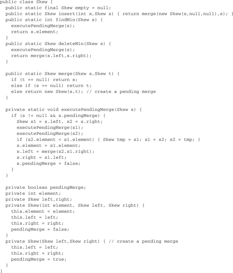
Figure 41.12Skew heaps with lazy evaluation in Java.
A crucial aspect of lazy evaluation is that a pending computation, once triggered, is executed only far enough to produce the part of the result that is needed. The remaining parts of the computation may be delayed further by creating new pending nodes. In the case of the merge operation, this means that when a pending merge is executed, the two roots are compared and the children of the smaller root are swapped as normal, but the recursive merge of the larger root with the former right child of the smaller root is not performed. Instead, a new pending merge is created and installed as the left child of the new root node. This process is illustrated in Figure 41.13, with the pending merges drawn as diamonds.
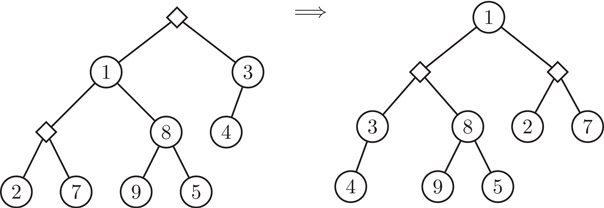
Figure 41.13Executing a pending merge.
Figure 41.14 illustrates the propagation of pending merges through a sequence of operations. First, the initial tree is built via a series of inserts. Then findMin executes those pending merges to find the value of the root. Next, deleteMin deletes the root and creates a new pending merge of the two children. Finally, findMin again executes the pending merges to find the new value of the root.
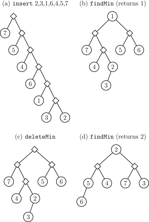
Figure 41.14A sequence of operations on skew heaps.
Notice that pending nodes and lazy evaluation affect when the various steps of a merge are carried out, but that they do not affect the end results of those steps. After all the pending merges have been executed, the final tree is identical to the one produced by skew heaps without lazy evaluation.
Strictly speaking, the nodes of a lazy skew heap can no longer be called immutable. In particular, when a pending merge is executed, the node representing the pending merge is updated with the result so that it cannot be executed twice. Functional languages typically allow this kind of mutation, known as memoization, because it is invisible to the user, except in terms of efficiency. Suppose that memoization was not performed. Then pending merges might be executed multiple times. However, every time a given pending merge was executed, it would produce the same result. Therefore, memoization is an optimization that makes lazy evaluation run faster, but that has no effect on the output of any computation.
41.4.1Analysis of Lazy Skew Heaps
Next, we prove that merge on lazy skew heaps runs in logarithmic amortized time. We use the banker’s method, associating a certain number of credits with each pending merge.
We begin with a few definitions. The logical view of a tree is what the tree would look like if all of its pending merges were executed. The logical left spine of a tree is the leftmost path from the root in the logical view. Similarly, the logical right spine of a tree is the rightmost path from the root in the logical view. A pending node is called left-heavy if its left subtree is at least as large as its right subtree in the logical view, or right-heavy if its right subtree is larger than its left subtree in the logical view. The successor of a pending node is the new pending node that is created as the new left child of the existing node when the existing node is executed.
Now, we charge one credit to execute a single pending merge. This credit pays for the comparison, the allocation of the successor node, and all necessary pointer manipulations, but it does not pay for executing the child nodes if they happen to be pending merges as well. When a right-heavy pending node is executed, it spends one of its own credits. When a left-heavy pending node is executed, the credit must be supplied either by its parent node, if it has one, or by the heap operation that originated the request, if the node is a root. This adds a single credit to the costs of the insert and deleteMin operations. After a pending node is executed, it passes any remaining credits to its successor node.
When we create a pending node, we must provide it with all the credits it will ever need. This includes
•One credit for itself, if it is right-heavy,
•One credit for each child that is a left-heavy pending node, and
•Any credits needed by its successors.
Notice that a pending node and its successors all lay on the logical left spine of the resulting tree in the logical view. Similarly, the physical children of a pending node and its successors all lay on the logical right spines of the argument trees to the original merge. Therefore, the number of credits that we must create during a merge is bounded by the number of right-heavy nodes in the logical left spine of the resulting tree plus the numbers of left-heavy nodes in the logical right spines of the argument trees.
It is easy to see that the number of right-heavy nodes in a logical left spine is at most logarithmic in the size of the logical view. Similarly, the number of left-heavy nodes in a logical right spine is at most logarithmic in the size of the logical view. The total number of credits created by merge is therefore bounded by the sum of three logarithmic values, and thus is logarithmic itself.
As this chapter has shown, many data structures work quite nicely in a functional setting. However, some do not. We close with a description of several warning signs to watch for.
•Random access: All of the data structures described in this chapter have been pointer-based. Unfortunately, data structures that depend on arrays—such as hash tables—are more difficult to handle. No entirely satisfactory approach is known for making arrays persistent. The best known approach from a theoretical point of view is that of Dietz [13], in which array accesses run in O(log log n) expected amortized time. However, his approach is quite complicated and difficult to implement. Competing approaches, such as [14–16], degrade to logarithmic (or worse!) time per access in common cases.
•Cycles: Not all pointer-based data structures are suitable for implementation in a functional setting. The most common problem is the presence of cycles, such as those found in doubly-linked lists or in binary search trees with parent pointers. Path copying requires copying all paths from the root to the site of the update. In the presence of cycles, this frequently means copying the entire data structure.
•Multiple entrypoints: Even without cycles, a pointer-based data structure can run into difficulties if it has multiple entrypoints. For example, consider a pointer-based implementation of the union-find data structure [17]. All the pointers go from children to parents, so there are no cycles (except sometimes trivial ones at the roots). However, it is common for every node of the union-find data structure to be a potential entrypoint, rather than just the root(s). Path copying requires copying all paths from any entrypoint to the site of the update. With multiple entrypoints, this again frequently degrades into copying the entire data structure.
•Unpredictable access patterns: Section 41.4 described how to use lazy evaluation to make an amortized data structure persistent. Although this works for many amortized data structures, such as skew heaps [12], it does not work for all amortized data structures. In particular, data structures with highly unpredictable access patterns, such as splay trees [18] (see Chapter 13), are difficult to make persistent in this fashion.
The most complete general reference on functional data structures is Okasaki [1]. For more information on specific data structures, consult the following sources:
•Priority queues and priority search queues [23,24]
•Random-access lists and flexible arrays [25–30]
•Catenable lists and deques [31–33]
This work was supported, in part, by the National Science Foundation under grant CCR-0098288. The views expressed in this chapter are those of the author and do not reflect the official policy or position of the United States Military Academy, the Department of the Army, the Department of Defense, or the U.S. Government.
1.C. Okasaki. Purely Functional Data Structures. Cambridge University Press, 1998.
2.S. Peyton Jones et al. Haskell 98: A non-strict, purely functional language. http://haskell.org/onlinereport/, Feb. 1999.
3.E. W. Myers. Efficient applicative data types. In ACM Symposium on Principles of Programming Languages, pages 66–75, Jan. 1984.
4.F. Rabhi and G. Lapalme. Algorithms: A Functional Programming Approach. Addison-Wesley, 1999.
5.C. Okasaki. Red-black trees in a functional setting. Journal of Functional Programming, 9(4):471–477, July 1999.
6.C. M. P. Reade. Balanced trees with removals: an exercise in rewriting and proof. Sci. Comput. Programming, 18(2):181–204, Apr. 1992.
7.S. Adams. Efficient sets—a balancing act. Journal of Functional Programming, 3(4):553–561, Oct. 1993.
8.R. Hinze. Explaining binomial heaps. Journal of Functional Programming, 9(1):93–104, Jan. 1999.
9.D. J. King. Functional binomial queues. In Glasgow Workshop on Functional Programming, pages 141–150. Sept. 1994.
10.M. Núñez, P. Palao, and R. Peña. A second year course on data structures based on functional programming. In Functional Programming Languages in Education, volume 1022 of LNCS, pages 65–84. Springer-Verlag, Dec. 1995.
11.C. Okasaki and A. Gill. Fast mergeable integer maps. In Workshop on ML, pages 77–86, Sept. 1998.
12.D. D. K. Sleator and R. E. Tarjan Self-adjusting heaps. SIAM Journal on Computing, 15(1):52–69, Feb. 1986.
13.P. F. Dietz. Fully persistent arrays. In Workshop on Algorithms and Data Structures, volume 382 of LNCS, pages 67–74. Springer-Verlag, Aug. 1989.
14.A. Aasa, S. Holmström, and C. Nilsson. An efficiency comparison of some representations of purely functional arrays. BIT, 28(3):490–503, 1988.
15.T. Chuang. A randomized implementation of multiple functional arrays. In ACM Conference on LISP and Functional Programming, pages 173–184, June 1994.
16.E. O’Neill and F. W. Burton A new method for functional arrays. Journal of Functional Programming, 7(5):487–513, Sept. 1997.
17.R. E. Tarjan. Data Structures and Network Algorithms, volume 44 of CBMS Regional Conference Series in Applied Mathematics. Society for Industrial and Applied Mathematics, Philadelphia, 1983.
18.D. D. K. Sleator and R. E. Tarjan. Self-adjusting binary search trees. Journal of the ACM, 32(3):652–686, July 1985.
19.T. Chuang and B. Goldberg. Real-time deques, multihead Turing machines, and purely functional programming. In Conference on Functional Programming Languages and Computer Architecture, pages 289–298, June 1993.
20.R. Hood. The Efficient Implementation of Very-High-Level Programming Language Constructs. PhD thesis, Department of Computer Science, Cornell University, Aug. 1982. (Cornell TR 82–503).
21.R. Hood and R. Melville. Real-time queue operations in pure Lisp. Information Processing Letters, 13(2):50–53, Nov. 1981.
22.C. Okasaki. Simple and efficient purely functional queues and deques. Journal of Functional Programming, 5(4):583–592, Oct. 1995.
23.G. S. Brodal and C. Okasaki. Optimal purely functional priority queues. Journal of Functional Programming, 6(6):839–857, Nov. 1996.
24.R. Hinze. A simple implementation technique for priority search queues. In ACM SIGPLAN International Conference on Functional Programming, pages 110–121, Sept. 2001.
25.R. Hinze. Bootstrapping one-sided flexible arrays. In ACM SIGPLAN International Conference on Functional Programming, pages 2–13, Sept. 2002.
26.R. R. Hoogerwoord. A logarithmic implementation of flexible arrays. In Conference on Mathematics of Program Construction, volume 669 of LNCS, pages 191–207. Springer-Verlag, July 1992.
27.A. Kaldewaij and V. J. Dielissen. Leaf trees. Science of Computer Programming, 26(1–3):149–165, May 1996.
28.E. W. Myers. An applicative random-access stack. Information Processing Letters, 17(5):241–248, Dec. 1983.
29.C. Okasaki. Purely functional random-access lists. In Conference on Functional Programming Languages and Computer Architecture, pages 86–95, June 1995.
30.C. Okasaki. Three algorithms on Braun trees. Journal of Functional Programming, 7(6):661–666, Nov. 1997.
31.H. Kaplan and R. E. Tarjan. Purely functional, real-time deques with catenation. Journal of the ACM, 46(5):577–603, Sept. 1999.
32.C. Okasaki. Amortization, lazy evaluation, and persistence: Lists with catenation via lazy linking. In IEEE Symposium on Foundations of Computer Science, pages 646–654, Oct. 1995.
33.C. Okasaki. Catenable double-ended queues. In ACM SIGPLAN International Conference on Functional Programming, pages 66–74, June 1997.
*This chapter has been reprinted from first edition of this Handbook, without any content updates.
†Actually, many functional languages do provide mechanisms for mutation, but their use is discouraged.
*Or higher-order functions, but we will not discuss higher-order functions further because they have relatively little effect on the implementation of data structures.