
Computational Geometry: Proximity and Location*
Sunil Arya
Hong Kong University of Science and Technology
David M. Mount
University of Maryland
Kirkpatrick’s Algorithm•Slab-Based Methods and Persistent Trees•Separating Chains and Fractional Cascading•Trapezoidal Maps and the History Graph•Worst- and Expected-Case Optimal Point Location
Voronoi Diagrams•Delaunay Triangulations•Other Geometric Proximity Structures
66.4Nearest Neighbor Searching
Nearest Neighbor Searching Through Point Location•K-d Trees•Other Approaches to Nearest Neighbor Searching•Approximate Nearest Neighbor Searching•Approximate Voronoi Diagrams
66.5Sources and Related Material
Proximity and location are fundamental concepts in geometric computation. The term proximity refers informally to the quality of being close to some point or object. Typical problems in this area involve computing geometric structures based on proximity, such as the Voronoi diagram, Delaunay triangulation and related graph structures such as the relative neighborhood graph. Another class of problems are retrieval problems based on proximity. These include nearest neighbor searching and the related concept of range searching. (See Chapter 19 for a discussion of data structures for range searching.) Instances of proximity structures and proximity searching arise in many fields of applications and in many dimensions. These applications include object classification in pattern recognition, document analysis, data compression, and data mining.
The term location refers to the position of a point relative to a geometric subdivision or a given set of disjoint geometric objects. The best known example is the point location problem, in which a subdivision of space into disjoint regions is given, and the problem is to identify which region contains a given query point. This problem is widely used in areas such as computer graphics, geographic information systems, and robotics. Point location is also used as a method for proximity searching, when applied in conjunction with Voronoi diagrams.
In this chapter we will present a number of geometric data structures that arise in the context of proximity and location. The area is so vast that our presentation will be limited to a relatively few relevant results. We will discuss data structures for answering point location queries first. After this we will introduce proximity structures, including Voronoi diagrams and Delaunay triangulations. Our presentation of these topics will be primarily restricted to the plane. Finally, we will present results on multidimensional nearest neighbor searching.
The planar point location problem is one of the most fundamental query problems in computational geometry. Consider a planar straight line graph S. (See Chapter 18 for details.) This is an undirected graph, drawn in the plane, whose edges are straight line segments that have pairwise disjoint interiors. The edges of S subdivide the plane into (possibly unbounded) polygonal regions, called faces. Henceforth, such a structure will be referred to as a polygonal subdivision. Throughout, we let n denote the combinatorial complexity of S, that is, the total number of vertices, edges and faces. (We shall occasionally abuse notation and use n to refer to the specific number of vertices, edges, or faces of S.) A planar subdivision is a special case of the more general topological concept of a cell complex [1], in which vertices, edges, and generally faces of various dimensions are joined together so that the intersection of any two faces is either empty or is a face of lower dimension.
The point location problem is to preprocess a polygonal subdivision S in the plane into a data structure so that, given any query point q, the polygonal face of the subdivision containing q can be reported quickly. (In Figure 66.1a, face A would be reported.) This problem is a natural generalization of the binary search problem in 1-dimensional space, where the faces of the subdivision correspond to the intervals between the 1-dimensional key values. By analogy with the 1-dimensional case, the goal is to preprocess a subdivision into a data structure of size O(n) so that point location queries can be answered in O(log n) time.
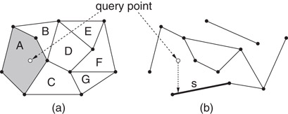
Figure 66.1Illustration of (a) point location and (b) vertical ray shooting queries.
A slightly more general formulation of the problem, which is applicable even when the input is not a subdivision is called vertical ray shooting. A set S of line segments is given with pairwise disjoint interiors. Given a query point q, the problem is to determine the line segment of S that lies vertically below q. (In Figure 66.1b, the segment s would be reported.) If the ray hits no segment, a special value is returned. When S is a polygonal subdivision, point location can be reduced to vertical ray shooting by associating each edge of S with the face that lies immediately above it.
Kirkpatrick was the first to present a simple point location data structure that is asymptotically optimal [2]. It answers queries in O(log n) time using O(n) space. Although this is not the most practical approach to point location, it is quite easy to understand.
Kirkpatrick starts with the assumption that the planar subdivision has been refined (through the addition of O(n) new edges and vertices) so that it is a triangulation whose external face is a triangle. Let T0 denote this initial triangulation subdivision. Kirkpatrick’s method generates a finite sequence of increasingly coarser triangulations, 〈T0, T1, T2, …, Tm〉, where Tm consists of the single triangle forming the outer face of the original triangulation. This sequence satisfies the following constraints: (a) each triangle of Ti+1 intersects a constant number of triangles of Ti, and (b) the number of vertices of Ti+1 is smaller than the number of vertices of Ti by a constant fraction. (See Figure 66.2.)
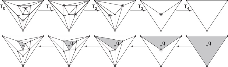
Figure 66.2The sequence of triangulations generated in the construction of Kirkpatrick’s structure (above) and the triangles visited in answering a point location query (below).
The data structure itself is a rooted DAG (directed acyclic graph), where the root of the structure corresponds to the single triangle of Tm, and the leaves correspond to the triangles of T0. The interior nodes of the DAG correspond to the triangles of each of the triangulations. A directed edge connects each triangle in Ti+1 with each triangle in Ti that it overlaps.
Given a query point q, the point location query proceeds level-by-level through the DAG, visiting the nodes corresponding to the triangles that contain q. By property (a), each triangle in Ti+1 overlaps a constant number of triangles of Ti, which implies that it is possible to descend one level in the data structure in O(1) time. It follows that the running time is proportional to the number of levels in the tree. By property (b), the number of vertices decreases at each level by a fixed constant fraction, and hence, the number of levels is O(log n). Thus the overall query time is O(log n).
Kirkpatrick showed how to build the data structure by constructing a sequence of triangulations satisfying the above properties. Kirkpatrick’s approach is to compute an independent set of vertices (that is, a set of mutually nonadjacent vertices) in Ti where each vertex of the independent set has constant degree. (An example is shown at the top of Figure 66.2. The vertices of the independent set are highlighted.) The three vertices of the outer face are not included. Kirkpatrick showed that there exists such a set whose size is a constant fraction of the total number of vertices, and it can be computed in linear time. These vertices are removed along with any incident edges, and the resulting “holes” are then retriangulated. Kirkpatrick showed that the two properties hold for the resulting sequence of triangulations.
66.2.2Slab-Based Methods and Persistent Trees
Many point location methods operate by refining the given subdivision to form one that is better structured, and hence, easier to search. One approach for generating such a refinement is to draw a vertical line through each vertex of the subdivision. These lines partition the plane into a collection of O(n) vertical slabs, such that there is no vertex within each slab. As a result, the intersection of the subdivision with each slab consists of a set of line segments, which cut clear through the slab. These segments thus partition the slab into a collection of disjoint trapezoids with vertical sides. (See Figure 66.3.)
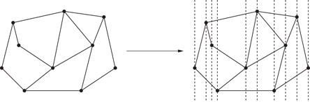
Figure 66.3Slab refinement of a subdivision.
Point location queries can be answered in O(log n) time by applying two binary searches. The first search accesses the query point’s x coordinate to determine the slab containing the query point. The second binary search tests whether the query point lies above or below individual lines of the slab, in order to determine which trapezoid contains the query point. Since each slab can be intersected by at most n lines, this second search can be done in O(log n) time as well.
A straightforward implementation of this method is not space efficient, since there are Ω(n) slabs,* each having up to Ω(n) intersecting segments, for a total of Ω(n2) space. However, adjacent slabs are very similar, since the only segments that change are those that are incident to the vertices lying on the slab boundary. Sarnak and Tarjan [4] exploited this idea to produce an optimal point location data structure. To understand their algorithm, imagine sweeping a line segment continuously from left to right. Consider the sorted order of subdivision line segments intersecting this sweep line. Whenever the sweep line encounters a vertex of the subdivision, the edges incident to this vertex lying to the left of the vertex are removed from the sweep-line order and incident edges to the right of the vertex are inserted. Since every edge is inserted once and deleted once in this process, the total number of changes over the entire sweep process is O(n).
Sarnak and Tarjan proposed maintaining a persistent variant of the search tree. A persistent search tree is a dynamic search tree (supporting insertion and deletion) which can answer queries not only to the current tree, but to any of the previous versions in the history of the tree’s lifetime as well. (See Chapter 33.) In this context, the history of changes to the search tree is maintained in a left to right sweep of the plane. The persistent search tree supports queries to any of these trees, that is, in any of the slabs, in O(log n) time. The clever aspect of Sarnak and Tarjan’s tree is that it can be stored in O(n) total space (as opposed to O(n2) space, which would result by generating O(n) copies of the tree). This is done by a method called limited node copying. Thus, this provides an asymptotically optimal point location algorithm. A similar approach was discovered independently by Cole [5].
66.2.3Separating Chains and Fractional Cascading
Slab methods use vertical lines to help organize the search. An alternative approach, first suggested by Lee and Preparata [6], is to use a divide-and-conquer approach based on a hierarchy of monotone polygon chains, called separating chains. A simple polygon is said to be x-monotone if the intersection of the interior of the polygon with a vertical line is connected. An x-monotone subdivision is one in which all the faces are x-monotone. The separating chain method requires that the input be an x-monotone subdivision. Fortunately, it is possible to convert any polygonal subdivision in the plane into an x-monotone subdivision in O(n log n) time, through the addition of O(n) new edges. (See e.g., [6–8].) For example, Figure 66.4a shows a subdivision that is not x-monotone, but the addition of two edges suffice to produce an x-monotone subdivision shown in Figure 66.4b.
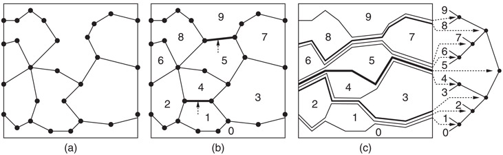
Figure 66.4Point location by separating chains: (a) the original subdivision, (b) the addition of one or more edges to make the subdivision x-monotone, (c) decomposition of the subdivision into a hierarchy of separating chains.
Consider an x-monotone subdivision with n faces. It is possible to order the faces f0, f1, …, fn−1 such that if i < j, then every vertical line that intersects both of these faces intersects fi below fj. (See Figure 66.4b.) For each i, 0 < i < n, define the ith separating chain to be the x-monotone polygonal chain separating faces whose indices are less than i from those that are greater than or equal to i.
Observe that, given a chain with m edges, it is possible to determine whether a given query point lies above or below the chain in O(log m) time, by first performing a binary search on the x-coordinates of the chain, in order to find which chain edge overlaps the query point, and then determining whether the query point lies above or below this edge in O(1) time. The separating chain method works intuitively by performing a binary search on these chains. The binary search can be visualized as a binary tree imposed on the chains, as shown in Figure 66.4c.
Although many chains traverse the same edge, it suffices to store each edge only once in the structure, namely with the chain associated with the highest node in the binary tree. This is because once a discrimination of the query point is made with respect to such an edge, its relation is implicitly known for all other chains that share the same edge. It follows that the total space is O(n).
As mentioned above, at each chain the search takes logarithmic time to determine whether the query point is above or below the chain. Since there are Ω(n) chains, this would lead to an Ω(log2n) algorithm [6]. There is a clever way to reduce the search time to O(log n), through the use of a simple and powerful method called fractional cascading [9,10]. Intuitively, fractional cascading seeks to replace a sequence of independent binary searches with a more efficient sequence of coordinated searches. After searching through a parent’s chain, it is known which edge of this chain the query point overlaps. Thus, it is not necessary to search the entire range of x-coordinates for the child’s chain, just the sublist of x-coordinates that overlap this interval.
However, in general, the number of edges of the child’s chain that overlaps this interval may be as large as Ω(n), and so this observation would seem to be of no help. In fractional cascading, this situation is remedied by augmenting each list. Starting with the leaf level, the x-coordinate of every fourth vertex is passed up from each child’s sorted list of x-coordinates and inserted into its parent’s list. This is repeated from the parent to the grandparent, and so on. After doing this, once the edge of the parent’s chain that overlaps the query point has been determined, there can be at most four edges of the child’s chain that overlap this interval. (e.g., in Figure 66.5 the edge is overlapped by eight edges at the next lower level. After cascading, it is broken into three subedges, each of which overlaps at most four edges at the next level.) Thus, the overlapping edge in the child’s chain can be found in O(1) time. The root requires O(log n) time, and each of the subsequent O(log n) searches can be performed in O(1) additional time. It can be shown that this augmentation of the lists increases the total size of all the lists by at most a constant factor, and hence the total space is still O(n).
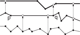
Figure 66.5Example of fractional cascading. Every fourth vertex is sampled from each chain and inserted in its parent’s chain.
66.2.4Trapezoidal Maps and the History Graph
Next we describe a randomized approach for point location. It is quite simple and practical. Let us assume that the planar subdivision is presented simply as a set of n line segments S = {s1, s2, …, sn} with pairwise disjoint interiors. The algorithm answers vertical ray-shooting queries as described earlier. This approach was developed by Mulmuley [11]. Also see Seidel [12].
The algorithm is based on a structure called a trapezoidal map (or trapezoidal decomposition). First, assume that the entire domain of interest is enclosed in a large rectangle. Imagine shooting a bullet vertically upwards and downwards from each vertex in the polygonal subdivision until it hits another segment of S. To simplify the presentation, we shall assume that the x-coordinates of no two vertices are identical. The segments of S together with the resulting bullet paths subdivide the plane into O(n) trapezoidal cells with vertical sides, which may degenerate to triangles. (See Figure 66.6a.)
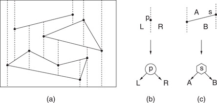
Figure 66.6A trapezoidal map of a set of segments (a), and the two types of internal nodes: x-node (b) and y-node (c).
For the purposes of point location, the trapezoidal map is created by a process called a randomized incremental construction. The process starts with the initial bounding rectangle (i.e., one trapezoid) and then the segments of S are inserted one by one in random order. As each segment is added, the trapezoidal map is updated by “walking” the segment through the subdivision, and updating the map by shooting new bullet paths through the segments endpoints and trimming existing paths that hit the new segment. See References 7,11,12 for further details. The number of changes in the diagram with each insertion is proportional to the number of vertical segments crossed by the newly added segment, which in the worst case may be as high as Ω(n). It can be shown, however, that on average each insertion of a new segment results in O(1) changes. This is true irrespective of the distribution of the segments, and the expectation is taken over all possible insertion orders.
The point location data structure is based on a rooted directed acyclic graph, or DAG, called the history DAG. Each node has either two outgoing edges (internal nodes) or none (leaves). Leaves correspond one-to-one with the cells of the trapezoidal map. There are two types of internal nodes, x-nodes and y-nodes. Each x-node contains the x-coordinate x0 of an endpoint of one of the segments, and its two children correspond to the points lying to the left and to the right of the vertical line x = x0. Each y-node contains a pointer to a line segment of the subdivision. The left and right children correspond to whether the query point is above or below the line containing this segment, respectively. (In Figure 66.7, x-nodes are shown as circles, y-nodes as hexagons, and leaves as squares.)
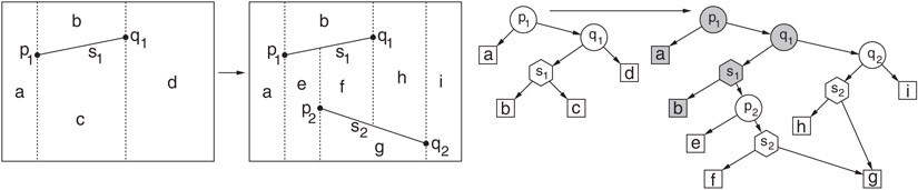
Figure 66.7Example of incremental construction of a trapezoidal map and the associated history DAG. The insertion of segment s2 replaces the leaves associated with destroyed trapezoids c and d with an appropriate search structure for the new trapezoids e–i.
As with Kirkpatrick’s algorithm, the construction of the point location data structure encodes the history of the randomized incremental construction. Let 〈T0, T1, …, Tn〉 denote the sequence of trapezoidal maps that result through the randomized incremental process. The point location structure after insertion of the ith segment has one leaf for each trapezoid in Ti. Whenever a segment is inserted, the leaf nodes corresponding to trapezoids that were destroyed are replaced with internal x- and y-nodes that direct the search to the location of the query point in the newly created trapezoids, after the insertion. (This is illustrated in Figure 66.7.) Through the use of node sharing, the resulting data structure can be shown to have expected size O(n), and its expected depth is O(log n), where the expectation is over all insertion orders. Details can be found in References 7,11,12.
66.2.5Worst- and Expected-Case Optimal Point Location
Goodrich, Orletsky and Ramaiyer [13] posed the question of bounding the minimum number of comparisons required, in the worst case, to answer point location queries in a subdivision of n segments. Adamy and Seidel [14] provided a definitive answer by showing that point location queries can be answered with primitive comparisons. They also gave a similar lower bound.
Another natural question involves the expected-case complexity of point location. Given a polygonal subdivision S, assume that each cell z ∈ S is associated with the probability pz that a query point lies in z. The problem is to produce a point location data structure whose expected search time is as low as possible. The appropriate target bound on the number of comparisons is given by the entropy of the subdivision, which is denoted by H and defined:
In the 1-dimensional case, a classical result due to Shannon implies that the expected number of comparisons needed to answer such queries is at least as large as the entropy of the probability distribution [15,16]. Mehlhorn [17] showed that in the 1-dimensional case it is possible to build a binary search tree whose expected search time is at most H + 2.
Arya, Malamatos, and Mount [18,19] presented a number of results on this problem in the planar case, and among them they showed that for a polygonal subdivision of size n in which each cell has constant combinatorial complexity, it is possible to answer point location queries with H + o(H) comparisons in the expected case using space that is nearly linear in n. Their results also applied to subdivisions with convex cells, assuming the query distribution is uniform within each cell. Their approach was loosely based on computing a binary space partition (BSP) tree (see Chapter 21) satisfying two properties:
1.The entropy of the subdivision defined by the leaves of the BSP should be close to the entropy of the original subdivision.
2.The depth of a leaf should be close to log2 (1/p), where p is the probability that a query point lies within the leaf.
Arya, Malamatos, and Mount [20] also presented a simple weighted variant of the randomized incremental algorithm and showed that it can answer queries in O(H) expected time and O(n) space. Iacono [21] presented a deterministic weighted variant based on Kirkpatrick’s algorithm.
Proximity structures arise from numerous applications in science and engineering. It is a fundamental fact that nearby objects tend to exert a greater influence and have greater relevance than more distant objects. Proximity structures are discrete geometric and graph structures that encode proximity information. We discuss a number of such structures, including Voronoi diagrams, Delaunay triangulations, and various geometric graph structures, such as the relative neighborhood graph.
The Voronoi diagram of a set of sites S is a partition of space into regions, one per site, where the region for site s is the set of points that are closer to s than to any other site of S. This structure has been rediscovered and applied in many different branches of science and goes by various names, including Thiessen diagrams and Dirichlet tessellations.
Henceforth, we consider the most common case in which the sites S consist of a set of n points in real d-dimensional space, , and distances are measured using the Euclidean metric. The set of points of that are closer to some site s ∈ S than any other site is called the Voronoi cell of s, or V (s). (See Figure 66.8.) The union of the boundaries of the Voronoi cells is the Voronoi diagram of S, denoted Vor(S). Observe that the set of points of that are closer to s than some other site t consists of the points that lie in the open halfspace defined by a plane that bisects the pair (s, t). It follows that each Voronoi cell is the intersection of n − 1 halfspaces, and hence, it is a (possibly unbounded) convex polyhedron. A Voronoi diagram in dimension d is a cell complex whose faces of all dimensions are convex polyhedra. In the plane a Voronoi diagram is a planar straight line graph with possibly unbounded edges. It can be represented using standard methods for representing polygonal subdivisions and cell complexes (see Chapter 18).
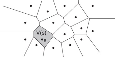
Figure 66.8The Voronoi diagram and a Voronoi cell V (s).
The Voronoi diagram possesses a number of useful geometric properties. For example, for a set of points in the plane, each edge of the Voronoi diagram lies on the perpendicular bisector between two sites. The vertices of the Voronoi diagram lie at the center of an empty circle passing through the incident sites. If the points are in general position (and in particular if no four points are cocircular) then every vertex of the diagram is incident to exactly three edges. In fact, it is not hard to show that the largest empty circle whose center lies within the convex hull of a given point set will coincide with a Voronoi vertex. In higher dimensions, each face of dimension k of the Voronoi diagram consists of the points of that are equidistant from a subset of d − k + 1 sites, and all other sites are strictly farther away. In the plane the combinatorial complexity of the Voronoi diagram is O(n), and in dimension d its complexity is .
Further information on algorithms for constructing Voronoi diagrams as well as variants of the Voronoi diagram can be found in Chapter 65. Although we defined Voronoi diagrams for point sites, it is possible to define them for any type of geometric object. One such variant involves replacing point sites with line segments or generally the boundary of any region of the plane. Given a region P (e.g., a simple polygon), the medial axis is defined to be the set of centers of maximal balls contained in P, that is, balls contained in P that are not contained in another ball in P [22]. The medial axis is frequently used in pattern recognition and shape matching. It consists of a combination of straight-line segments and hyperbolic arcs. It can be computed in O(n log n) time by a modification of Fortune’s sweepline algorithm [23]. Finally, it is possible to generalize Voronoi diagrams to other metrics, such as the L1 and L∞ metrics (see Section 66.4).
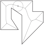
The Delaunay triangulation is a structure that is closely related to the Voronoi diagram. The Delaunay triangulation is defined as follows for a set S of n point sites in the plane. Consider any subset T ⊆ S of sites, such that there exists a circle that passes through all the points of T, and contains no point of S in its interior. Such a subset is said to satisfy the empty circumcircle property. For example, in Figure 66.9a, the pair {p, q} and triple {r, s, t} both satisfy the empty circumcircle property. The Delaunay triangulation is defined to be the union of the convex hulls of all such subsets. It can be shown that the result is a cell complex. Furthermore, if the points are in general position, and in particular, no four points are cocircular, then the resulting structure is a triangulation of S. (If S is not in general position, then some faces may have more than three edges, and it is common to complete the triangulation by triangulating each such face.) A straightforward consequence of the above definition is that the Delaunay triangulation is dual to the Voronoi diagram. For example, Figure 66.9b shows the overlay of these two structures in the plane.
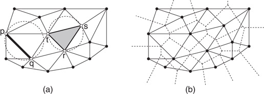
Figure 66.9(a) The Delaunay triangulation of a set of points and (b) its overlay with the Voronoi diagram.
Delaunay triangulations are widely used in practice, and they possess a number of useful properties. For example, among all triangulations of a planar point set the Delaunay triangulation maximizes the minimum angle. Also, in all dimensions, the Euclidean minimum spanning tree (defined below) is a subgraph of the Delaunay triangulation. Proofs of these facts can be found in Reference 7.
In the plane the Delaunay triangulation of a set of points has O(n) edges and O(n) faces. The above definition can be generalized to arbitrary dimensions. In dimension d, the Delaunay triangulation can have as many as faces. However, it can be much smaller. In particular, Dwyer [24] has shown that in any fixed dimension, if n points are drawn from a uniform distribution from within a unit ball, then the expected number of simplices is O(n).
There is an interesting connection between Delaunay triangulations in dimension d and convex hulls in dimension d + 1. Consider the lifting map defined f(x, y) = (x, y, x2 + y2). This projects points in the plane onto the paraboloid z = x2 + y2. Given a planar point set S, let S′ denote the set of points of that results by applying this map to each point of S. Define the lower hull of S′ to be the set of faces whose outward pointing normal has a negative z coordinate. It can be shown that, when projected back to the plane, the edges of the lower convex hull of S′ are exactly the edges of the Delaunay triangulation of S. (See Figure 66.10.)
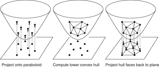
Figure 66.10The Delaunay triangulation can be computed by lifting the points to the paraboloid, computing the lower convex hull, and projecting back to the plane.
Although there exist algorithms specially designed for computing Delaunay triangulations, the above fact makes it possible to compute Delaunay triangulations in any dimension by computing convex hulls in the next higher dimension. There exist O(n log n) time algorithms for computing planar Delaunay triangulations, for example, based on divide-and-conquer [25] and plane sweep [23]. Perhaps the most popular method is based on randomized incremental point insertion [26]. In dimension d ≥ 3, Delaunay triangulations can be computed in time through randomized incremental point insertion [27].
66.3.3Other Geometric Proximity Structures
The Delaunay triangulation is perhaps the best known example of a proximity structure. There are a number of related graph structures that are widely used in pattern recognition, learning, and other applications. Given a finite set S of points in d-dimensional Euclidean space, we can define a graph on these points by joining pairs of points that satisfy certain neighborhood properties. In this section we will consider a number of such neighborhood graphs.
Let us first introduce some definitions. For let dist(p, q) denote the Euclidean distance from p to q. Given positive , let B(p, r) be the open ball consisting of points whose distance from point p is strictly less than r. Define the lune, denoted L(p, q), to be the intersection of two balls both of radius dist(p, q) centered at these points, that is,
The following geometric graphs are defined for a set S consisting of n points in . (See Figure 66.11.)
Figure 66.11Common geometric graphs on a point set.
Nearest Neighbor Graph (NNG): The directed graph containing an edge (p, q) if q is the nearest neighbor of p, that is, B(p, dist(p, q)) ∩ S = θ.
Euclidean Minimum Spanning Tree (EMST): This is an undirected spanning tree on S that minimizes the sum of the Euclidean edge lengths.
Relative Neighborhood Graph (RNG): The undirected graph containing an edge (p, q) if there is no point r ∈ S that is simultaneously closer to p and q than dist(p, q) [28]. Equivalently, (p, q) is an edge if L(p, q) ∩ S = θ.
Gabriel Graph (GG): The undirected graph containing an edge (p, q) if the ball whose diameter is does not contain any other points of S [29], that is, if
Delaunay Graph (DT): The 1-skeleton (edges) of the Delaunay triangulation.
These graphs form an interesting hierarchical relationship. If we think of each edge of an undirected graph as consisting of two directed edges, then we have the following hierarchical relationship, which was first established in Reference 28. Also see Reference 30.
This holds in all finite dimensions and generalizes to Minkowski (Lm) metrics, as well.
66.4Nearest Neighbor Searching
Nearest neighbor searching is an important problem in a variety of applications, including knowledge discovery and data mining, pattern recognition and classification, machine learning, data compression, multimedia databases, document retrieval, and statistics. We are given a set S of objects in some space to be preprocessed, so that given a query object q, the closest object (or objects) of S can be reported quickly.
There are many ways in which to define the notion of similarity. Because the focus of this chapter is on geometric approaches, we shall assume that proximity is defined in terms of the well known Euclidean distance. Most of the results to be presented below can be generalized to any Minkowski (or Lm) metric, in which the distance between two points p and q is defined to be
where m ≥ 1 is a constant. The case m = 2 is the Euclidean distance, the case m = 1 is the Manhattan distance, and the limiting case m = ∞ is the max distance. In typical geometric applications the dimension d is assumed to be a fixed constant. There has also been work on high dimensional proximity searching in spaces of arbitrarily high dimensions [31] and in arbitrary (nongeometric) metric spaces [32], which we shall not cover here.
There are a number of natural extensions to the nearest neighbor problem as described above. One is to report the k nearest neighbors to the query point, for some given integer k. Another is to compute all the points lying within some given distance, that is, a range query in which the range is defined by the distance function.
Obviously, without any preprocessing whatsoever, the nearest neighbor search problem can be solved in O(n) time through simple brute-force search. A number of very simple methods have been proposed which assume minimal preprocessing. For example, points can be sorted according to their projection along a line, and the projected distances can be used as a method to prune points from consideration [33–35]. These methods are only marginally effective, and provide significant improvements over brute-force search only in very low dimensions.
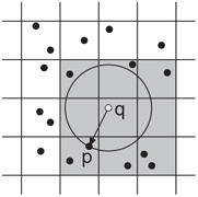
For uniformly distributed point sets, good expected case performance can be achieved by simple decompositions of space into a regular grid of hypercubes. Rivest [36] and later Cleary [37] provided analyses of these methods. Bentley, Weide, and Yao [38] also analyzed a grid-based method for distributions satisfying certain bounded-density assumptions. Intuitively, the points are bucketed into grid cells, where the size of the grid cell is based on the expected distance to the nearest neighbor. To answer a query, the grid cell containing the query point is located, and a spiral-like search working outwards from this cell is performed to identify nearby points. Suppose for example that q is the query point and p is its closest neighbor. Then all the grid cells overlapping a ball centered at q of radius dist(p, q) would be visited.
Grids are easy to implement, since each bucket can be stored as a simple list of points, and the complete set of buckets can be arranged in a multi-dimensional array. Note that this may not be space efficient, since it requires storage for empty cells. A more space-efficient method is to assign a hash code to each grid cell based on its location, and then store only the nonempty grid buckets in a hash table. In general, grid methods do not work well for nearest neighbor search unless the point distribution is roughly uniform. As will be discussed below, more sophisticated methods are needed to achieve good efficiency for nonuniformly distributed data.
66.4.1Nearest Neighbor Searching Through Point Location
One of the original motivations for the Voronoi diagram is nearest neighbor searching. By definition, the Voronoi diagram subdivides space into cells according to which site is the closest. So, in order to determine the closest site, it suffices to compute the Voronoi diagram and generate a point location data structure for the Voronoi diagram. In this way, nearest neighbor queries are reduced to point location queries. This provides an optimal O(n) space and O(log n) query time method for answering point location queries in the plane. Unfortunately, this solution does not generalize well to higher dimensions. The worst-case combinatorial complexity of the Voronoi diagram in dimension d grows as , and optimal point location data structures are not known to exist in higher dimensions.
Perhaps the most popular class of approaches to nearest neighbor searching involves some sort of hierarchical spatial subdivision. Let S denote the set of n points in for which queries are to be answered. In such an approach, the entire space is subdivided into successively smaller regions, and the resulting hierarchy is represented by a rooted tree. Each node of the tree represents a region of space, called a cell. Implicitly, each node represents the subset of points of S that lie within its cell. The root of the tree is associated with the entire space and the entire point set S. For some arbitrary node u of the tree, if the number of points of S associated with u is less than some constant, then this node is declared to be a leaf of the tree. Otherwise, the cell associated with u is recursively subdivided into smaller (possibly overlapping) subcells according to some splitting rule. Then the associated points of S are distributed among these children according to which subcell they lie in. These subcells are then associated with the children of u in the tree.
There are many ways in which to define such a subdivision. Perhaps the earliest and best known example is that of the k-d tree data structure. Bentley [39] introduced the k-d tree data structure (or kd-tree) as a practical general-purpose data structure for many types of geometric retrieval problems. Although it is not the asymptotically most efficient solution for these problems, its flexibility makes it a popular choice for implementation. The cells of a k-d tree are axis-aligned hyperrectangles. Each internal node is associated with an axis-orthogonal splitting hyperplane. This hyperplane splits the rectangular cell into two rectangular subcells, each of which is associated with one of the two children. An example is shown in Figure 66.12.
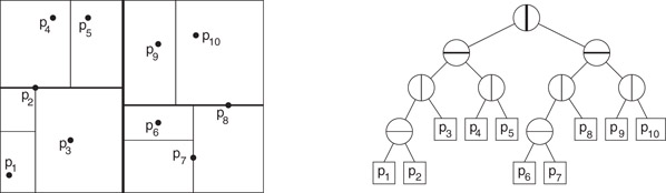
Figure 66.12An example of a k-d tree of a set of points in the plane, showing both the associated spatial subdivision (left) and the binary tree structure (right).
The choice of the splitting hyperplane is an important issue in the implementation of the k-d tree. For the purpose of nearest neighbor searching, a good split is one that divides the points into subsets of similar cardinalities and which produces cells that are not too skinny, that is, the ratio between the longest and shortest sides is bounded. However, it is not always possible to achieve these goals. A simple and commonly used method is to cycle through the various coordinate axes (i.e., splitting along x, then y, then z, then back to x, and so on). Each time the split is made through the median coordinate along the splitting dimension [7,40]. Friedman, Bentley and Finkel [41] suggested the following method, which is more sensitive to the data distribution. First, compute the minimum axis-aligned bounding box for the set of points associated with the current cell. Next choose the splitting axis to be the one that is parallel to the longest side of this box. Finally, split the points by a hyperplane that is orthogonal to this axis, and which splits the points into two sets of equal size. A number of other splitting rules have been proposed for k-d trees, including the sliding midpoint rule by Arya and Fu [42] and Maneewongvatana and Mount [43], variance minimization by White and Jain [44], and methods by Silva Filho [45] and Sproull [46]. We will discuss other subdivision methods in the next section as well.
It is possible to construct the k-d tree of an n-element point set in O(n log n) time by a simple top-down recursive procedure. The process involves determining the splitting axis and the splitting coordinate along this axis, and then partitioning the point set about this coordinate. If the splitting rule partitions the point set about its median coordinate then it suffices to compute the median by any linear-time algorithm for computing medians [3]. Some splitting methods may not evenly partition the point set. In the worst case this can lead to quadratic construction time. Vaidya showed that it is possible to achieve O(n log n) construction time, even when unbalanced splitting takes place [47]. The total space requirements are O(n) for the tree itself.
Given a query point q, a nearest neighbor search is performed by the following recursive algorithm [41]. Throughout, the algorithm maintains the closest point to q encountered so far in the search, and the distance to this closest point. As the nodes of the tree are traversed, the algorithm maintains the d-dimensional hyperrectangular cell associated with each node. (This is updated incrementally as the tree is traversed.) When the search arrives at a leaf node, it computes the distance from q to the associated point(s) of this node, and updates the closest point if necessary. (See Figure 66.13.) Otherwise, when it arrives at an internal node, it first computes the distance from the query point to the associated cell. If this distance is greater than the distance to the closest point so far, the search returns immediately, since the subtree rooted at this node cannot provide a closer point. Otherwise, it is determined which side of the splitting hyperplane contains the query point. First, the closer child is visited and then the farther child. A somewhat more intelligent variant of this method, called priority search, involves storing the unvisited nodes in a priority queue, sorted according to the distance from the query point to the associated cell, and then processes the nodes in increasing order of distance from the query point [48].
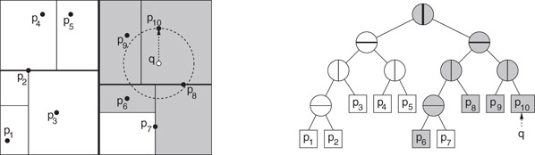
Figure 66.13Nearest neighbor search in a k-d tree. The point p10 is the initial closest, and only the shaded cells and nodes are visited. The final answer is p8.
66.4.3Other Approaches to Nearest Neighbor Searching
The k-d tree is but one example of a general class of nearest neighbor search structures that are based on hierarchical space decomposition. A good survey of methods from database literature was given by Böhm, Berchtold, and Keim [49]. These include the R-tree [50] and its variants, the R*-tree [51], the R+-tree [52], and the X-tree [53], which are all based on recursively decomposing space into (possibly overlapping) hyperrectangles. (See Chapter 22 for further information.) For the cases studied, the X-tree is reported to have the best performance for nearest neighbor searching in high dimensional spaces [49]. The SS-tree [44] is based on subdividing space using (possibly overlapping) hyperspheres rather than rectangles. The SR-tree [54] uses the intersection of an enclosing rectangle and enclosing sphere to represent a cell. The TV-tree [55] applies a novel approach of considering projections of the data set onto higher dimensional subspaces at successively deeper levels in the search tree.
A number of algorithms for nearest neighbor searching have been proposed in the algorithms and computational geometry literature. Higher dimensional solutions with sublinear worst-case performance were considered by Yao and Yao [56]. Clarkson [57] showed that queries could be answered in O(log n) time with space, for any δ > 0. The O-notation hides constant factors that are exponential in d. Agarwal and Matoušek [58] generalized this by providing a tradeoff between space and query time. Meiser [59] showed that queries could be answered in O(d5 log n) time and O(nd+δ) space, for any δ > 0, thus showing that exponential factors in query time could be eliminated by using sufficient space.
66.4.4Approximate Nearest Neighbor Searching
In any fixed dimensions greater than two, no method for exact nearest neighbor searching is known that achieves the simultaneous goals of roughly linear space and logarithmic query time. For methods achieving roughly linear space, the constant factors hidden in the asymptotic running time grow at least as fast as 2d (depending on the metric). Arya et al. [60] showed that if n is not significantly larger than 2d, then boundary effects decrease this exponential dimensional dependence. Nonetheless, the so called “curse of dimensionality” is a significant impediment to computing nearest neighbors efficiently in high dimensional spaces.
This suggests the idea of computing nearest neighbors approximately. Consider a set of points S and a query point q. For any ε > 0, we say that a point p ∈ S is an ε-approximate nearest neighbor of q if
where p* is the true nearest neighbor of q in S. The approximate nearest neighbor problem was first considered by Bern [61]. He proposed a data structure that achieved a fixed approximation factor depending on dimension. Arya and Mount [62] proposed a randomized data structure that achieves polylogarithmic query time in the expected case, and nearly linear space. Their approach was based on a combination of the notion of neighborhood graphs, as described in Section 66.3.3, and skip lists. In their algorithm the approximation error factor ε is an arbitrary positive constant, which is given at preprocessing time.
Arya et al. [63] proposed a hierarchical spatial subdivision data structure, called the BBD-tree. This structure has the nice features of having O(n) size, O(log n) depth, and each cell has bounded aspect ratio, that is, the ratio between its longest and shortest side is bounded. They achieved this by augmenting the axis-aligned splitting operation of the k-d tree (see Figure 66.14a) with an additional subdivision operation called shrinking (see Figure 66.14b). A shrinking node is associated with an axis-aligned rectangle, and the two children correspond to the portions of space lying inside and outside of this rectangle, respectively. The resulting cells are either axis-aligned hyperrectangles, or the set-theoretic difference of two axis-aligned hyperrectangles. They showed that, in all fixed dimensions d and for ε > 0, it is possible to answer ε-nearest neighbor queries in O(log n) time using the BBD-tree. The hidden asymptotic constants in query time grow as (1/ε)d.
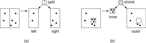
Figure 66.14Splitting nodes (a) and shrinking nodes (b) in a BBD-tree.
Duncan et al. [64] proposed an alternative structure, called the BAR tree, which achieves all of these combinatorial properties and has convex cells. The BAR tree achieves this by using cutting planes that are not necessarily axis-aligned. Clarkson [65] and Chan [66] presented data structures that achieved better ε dependency in the query time. In particular, they showed that queries could be answered in O((1/ε)d/2 log n) time.
66.4.5Approximate Voronoi Diagrams
As mentioned in Section 66.4.1 it is possible to answer nearest neighbor queries by applying a point location query to the Voronoi diagram. However, this approach does not generalize well to higher dimensions, because of the rapid growth rate of the Voronoi diagram and the lack of good point location structures in dimension higher than two.
Har-Peled [67] proposed a method to overcome these problems. Given an error bound ε > 0, an approximate Voronoi diagram (AVD) of a point set S is defined to be a partition of space into cells, where each cell c is associated with a representative rc ∈ S, such that rc is an ε-nearest neighbor for all the points in c [67]. Arya and Malamatos [68] generalized this by allowing up to some given number t ≥ 1 representatives to be stored with each cell, subject to the requirement that for any point in the cell, one of these t representatives is an ε-nearest neighbor. Such a decomposition is called a (t, ε)-AVD. (See Figure 66.15.)
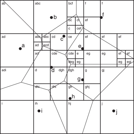
Figure 66.15A (3, 0)-AVD implemented as a quadtree subdivision for the set {a, b, …, j}. Each cell is labeled with its representatives. The Voronoi diagram is shown for reference.
Of particular interest are AVDs that are constructed from hierarchical spatial decompositions, such as quadtrees and their variants, since such structures support fast point location in all dimensions. This yields a very simple method for performing approximate nearest neighbor searching. In particular, a tree descent determines the leaf cell containing the query point and then the closest of the t representatives is reported.
Har-Peled [67] showed that it is possible to construct a (1, ε) AVD in which the number of leaf cells is O((n/εd)(log n) log (n/ε)). Arya and Malamatos [68] and later Arya, Malamatos, and Mount [69] improved these results by showing how to construct more space-efficient AVDs. In all constant dimensions d, their results yield a data structure of O(n) space (including the space for representatives) that can answer ε-nearest neighbor queries in O(log n + (1/ε)(d−1)/2) time. This is the best asymptotic result known for approximate nearest neighbor searching in fixed dimensional spaces.
66.5Sources and Related Material
General information regarding the topics presented in the chapter can be found in standard texts on computational geometry, including those by Preparata and Shamos [8], Edelsbrunner [1], Mulmuley [70], de Berg et al. [7], and Boissonnat and Yvinec [71] as well as Samet’s book on spatial data structures [40]. Further information on point location can be found in a survey paper written by Snoeyink [72]. For information on Voronoi diagrams see the book by Okabe, Boots and Sugihara [73] or surveys by Aurenhammer [74], Aurenhammer and Klein [75], and Fortune [76]. For further information on geometric graphs see the survey by O’Rourke and Toussaint [77]. Further information on nearest neighbor searching can be found in surveys by Böhm et al. [49], Indyk [31], and Chavez et al. [32].
The work of the first author was supported in part by a grant from the Hong Kong Research Grants Council (HKUST6229/00E and HKUST6080/01E). The work of the second author was supported in part by National Science Foundation grant number CCR-0098151.
1.H. Edelsbrunner: Algorithms in Combinatorial Geometry, Volume 10 of EATCS Monographs on Theoretical Computer Science. Springer-Verlag, Heidelberg, West Germany, 1987.
2.D. G. Kirkpatrick: Optimal search in planar subdivisions. SIAM J. Comput., 12(1):28–35, 1983.
3.T. H. Cormen, C. E. Leiserson, R. L. Rivest, and C. Stein: Introduction to Algorithms. MIT Press, Cambridge, MA, 2nd edition, 2001.
4.N. Sarnak and R. E. Tarjan: Planar point location using persistent search trees. Commun. ACM, 29(7):669–679, July 1986.
5.R. Cole: Searching and storing similar lists. J. Algorithms, 7:202–220, 1986.
6.D. T. Lee and F. P. Preparata: Location of a point in a planar subdivision and its applications. SIAM J. Comput., 6(3):594–606, 1977.
7.M. de Berg, M. van Kreveld, M. Overmars, and O. Schwarzkopf: Computational Geometry: Algorithms and Applications. Springer-Verlag, Berlin, Germany, 2nd edition, 2000.
8.F. P. Preparata and M. I. Shamos: Computational Geometry: An Introduction. Springer-Verlag, New York, 3rd edition, October 1990.
9.B. Chazelle and L. J. Guibas: Fractional cascading: I. A data structuring technique. Algorithmica, 1(3):133–162, 1986.
10.H. Edelsbrunner, L. J. Guibas, and J. Stolfi: Optimal point location in a monotone subdivision. SIAM J. Comput., 15(2):317–340, 1986.
11.Mulmuley, K.: A fast planar partition algorithm, I. J. Symbolic Comput., 10(3–4):253–280, 1990.
12.R. Seidel: A simple and fast incremental randomized algorithm for computing trapezoidal decompositions and for triangulating polygons. Comput. Geom. Theory Appl., 1(1):51–64, 1991.
13.Goodrich, M. T., M. Orletsky, and K. Ramaiyer: Methods for achieving fast query times in point location data structures. In Proc. 8th ACM-SIAM Sympos. Discrete Algorithms, pp. 757–766, 1997.
14.U. Adamy and R. Seidel: Planar point location close to the information-theoretic lower bound. In Proc. 9th ACM-SIAM Sympos. Discrete Algorithms, 1998.
15.D. E. Knuth: Sorting and Searching, Volume 3 of The Art of Computer Programming. Addison-Wesley, Reading, MA, second edition, 1998.
16.C. E. Shannon: A mathematical theory of communication. Bell Sys. Tech. Journal, 27:379–423, 623–656, 1948.
17.K. Mehlhorn: Best possible bounds on the weighted path length of optimum binary search trees. SIAM J. Comput., 6:235–239, 1977.
18.S. Arya, T. Malamatos, and D. M. Mount: Nearly optimal expected-case planar point location. In Proc. 41 Annu. IEEE Sympos. Found. Comput. Sci., pp. 208–218, 2000.
19.S. Arya, T. Malamatos, and D. M. Mount: Entropy-preserving cuttings and space-efficient planar point location. In Proc. 12th ACM-SIAM Sympos. Discrete Algorithms, pp. 256–261, 2001.
20.S. Arya, T. Malamatos, and D. M. Mount: A simple entropy-based algorithm for planar point location. In Proc. 12th ACM-SIAM Sympos. Discrete Algorithms, pp. 262–268, 2001.
21.J. Iacono: Optimal planar point location. In Proc. 12th ACM-SIAM Sympos. Discrete Algorithms, pp. 340–341, 2001.
22.Duda, R. O. and P. E. Hart: Pattern Classification and Scene Analysis. Wiley-Interscience, New York, 1973.
23.S. J. Fortune: A sweepline algorithm for Voronoi diagrams. Algorithmica, 2:153–174, 1987.
24.Dwyer, R. A.: Higher-dimensional Voronoi diagrams in linear expected time. Discrete Comput. Geom., 6:343–367, 1991.
25.M. I. Shamos and D. Hoey: Closest-point problems. In Proc. 16th Annu. IEEE Sympos. Found. Comput. Sci., pp. 151–162, 1975.
26.L. J. Guibas, D. E. Knuth, and M. Sharir: Randomized incremental construction of Delaunay and Voronoi diagrams. Algorithmica, 7:381–413, 1992.
27.K. L. Clarkson and P. W. Shor: Applications of random sampling in computational geometry II. Discrete Comput. Geom., 4:387–421, 1989.
28.G. T. Toussaint: The relative neighbourhood graph of a finite planar set. Pattern Recogn., 12:261–268, 1980.
29.K. R. Gabriel and R. R. Sokal: A new statistical approach to geographic variation analysis. Systematic Zoology, 18:259–278, 1969.
30.J. W. Jaromczyk and G. T. Toussaint: Relative neighborhood graphs and their relatives. Proc. IEEE, 80(9):1502–1517, September 1992.
31.A. Andoni and P. Indyk: Nearest neighbors in high-dimensional spaces. In J. E. Goodman, J. O’Rourke, and C. D. Toth, editors, Handbook of Discrete and Computational Geometry, 3rd edition, CRC Press LLC, Boca Raton, FL, 2017.
32.E. Chavez, G. Navarro, R. A. Baeza-Yates, and J. L. Marroquin: Searching in metric spaces. ACM Comput. Surveys, 33:273–321, 2001.
33.J. H. Friedman, F. Baskett, and L. J. Shustek: An algorithm for finding nearest neighbors. IEEE Trans. Comput., C-24(10):1000–1006, 1975.
34.L. Guan and M. Kamel: Equal-average hyperplane partitioning method for vector quantization of image data. Pattern Recogn. Lett., 13:693–699, 1992.
35.C.-H. Lee and L.-H. Chen: Fast closest codeword search algorithm for vector quantisation. IEE Proc.-Vis. Image Signal Process., 141:143–148, 1994.
36.R. L. Rivest: On the optimality of Elias’s algorithm for performing best-match searches. In Information Processing, pp. 678–681. North Holland Publishing Company, 1974.
37.Cleary, J. G.: Analysis of an algorithm for finding nearest neighbors in Euclidean space. ACM Trans. on Math. Softw., 5(2):183–192, 1979.
38.J. L. Bentley, B. W. Weide, and A. C. Yao: Optimal expected-time algorithms for closest point problems. ACM Trans. on Math. Softw., 6(4):563–580, 1980.
39.J. L. Bentley: Multidimensional binary search trees used for associative searching. Commun. ACM, 18(9):509–517, September 1975.
40.H. Samet: The Design and Analysis of Spatial Data Structures. Addison-Wesley, Reading, MA, 1990.
41.J. H. Friedman, J. L. Bentley, and R. A. Finkel: An algorithm for finding best matches in logarithmic expected time. ACM Trans. Math. Softw., 3:209–226, 1977.
42.S. Arya and H. Y. Fu: Expected-case complexity of approximate nearest neighbor searching. SIAM J. of Comput., 32:793–815, 2003.
43.S. Maneewongvatana and D. M. Mount: Analysis of approximate nearest neighbor searching with clustered point sets. In M. H. Goldwasser, C. C. McGeoch, and D. S. Johnson, editors, Data Structures, Near Neighbor Searches, and Methodology, Volume 59 of DIMACS Series in Discrete Mathematics and Theoretical Computer Science, pp. 105–123. American Mathematics Society, Providence, Rhode Island, 2002.
44.D. A. White and R. Jain: Similarity indexing with the SS-tree. In Proc. 12th IEEE Internat. Conf. Data Engineering, pp. 516–523, 1996.
45.Silva Filho, Y. V.: Optimal choice of discriminators in a balanced K-D binary search tree. Inform. Proc. Lett., 13:67–70, 1981.
46.R. F. Sproull: Refinements to nearest-neighbor searching in k-dimensional trees. Algorithmica, 6(4):579–589, 1991.
47.P. M. Vaidya: An O(n log n) algorithm for the all-nearest-neighbors problem. Discrete Comput. Geom., 4:101–115, 1989.
48.S. Arya and D. M. Mount: Algorithms for fast vector quantization. In Data Compression Conference, pp. 381–390. IEEE Press, 1993.
49.C. Böhm, S. Berchtold, and D. A. Keim: Searching in high-dimensional spaces: Index structures for improving the performance of multimedia databases. ACM Comput. Surveys, 33:322–373, 2001.
50.A. Guttman: R-trees: A dynamic index structure for spatial searching. In Proc. ACM SIGMOD Conf. on Management of Data, pp. 47–57, 1984.
51.N. Beckmann, H.-P. Kriegel, R. Schneider, and B. Seeger: The R*-tree: An efficient and robust access method for points and rectangles. In Proc. ACM SIGMOD Conf. on Management of Data, pp. 322–331, 1990.
52.T. Sellis, N. Roussopoulos, and C. Faloutsos: The R+ -tree: A dynamic index for multi-dimensional objects. In Proc. 13th VLDB Conference, pp. 507–517, 1987.
53.S. Berchtold, D. A. Keim, and H.-P. Kriegel: The X-tree: An index structure for high-dimensional data. In Proc. 22nd VLDB Conference, pp. 28–39, 1996.
54.N. Katayama and S. Satoh: The SR-tree: An index structure for high-dimensional nearest neighbor queries. In Proc. ACM SIGMOD Conf. on Management of Data, pp. 369–380, 1997.
55.K. I. Lin, H. V. Jagadish, and C. Faloutsos: The TV-tree: An index structure for high-dimensional data. VLDB Journal, 3(4):517–542, 1994.
56.A. C. Yao and F. F. Yao: A general approach to d-dimensional geometric queries. In Proc. 17th Ann. ACM Sympos. Theory Comput., pp. 163–168, 1985.
57.K. L. Clarkson: A randomized algorithm for closest-point queries. SIAM J. Comput., 17(4):830–847, 1988.
58.P. K. Agarwal and J. Matoušek: Ray shooting and parametric search. SIAM J. Comput., 22(4):794–806, 1993.
59.S. Meiser: Point location in arrangements of hyperplanes. Information and Computation, 106(2):286–303, 1993.
60.S. Arya, D. M. Mount, and O. Narayan: Accounting for boundary effects in nearest-neighbor searching. Discrete Comput. Geom., 16:155–176, 1996.
61.M. Bern: Approximate closest-point queries in high dimensions. Inform. Process. Lett., 45:95–99, 1993.
62.S. Arya and D. M. Mount: Approximate nearest neighbor queries in fixed dimensions. In Proc. 4th ACM-SIAM Sympos. Discrete Algorithms, pp. 271–280, 1993.
63.S. Arya, D. M. Mount, N. S. Netanyahu, R. Silverman, and A. Wu: An optimal algorithm for approximate nearest neighbor searching in fixed dimensions. J. ACM, 45:891–923, 1998.
64.C. A. Duncan, M. T. Goodrich, and S. Kobourov: Balanced aspect ratio trees: Combining the advantages of k-d trees and octrees. J. Algorithms, 38:303–333, 2001.
65.K. L. Clarkson: An algorithm for approximate closest-point queries. In Proc. 10th Annu. ACM Sympos. Comput. Geom., pp. 160–164, 1994.
66.T. Chan: Approximate nearest neighbor queries revisited. In Proc. 13th Annu. ACM Sympos. Comput. Geom., pp. 352–358, 1997.
67.S. Har-Peled: A replacement for Voronoi diagrams of near linear size. In Proc. 42 Annu. IEEE Sympos. Found. Comput. Sci., pp. 94–103, 2001.
68.S. Arya and T. Malamatos: Linear-size approximate Voronoi diagrams. In Proc. 13th ACM-SIAM Sympos. Discrete Algorithms, pp. 147–155, 2002.
69.S. Arya, T. Malamatos, and D. M. Mount: Space-efficient approximate Voronoi diagrams. In Proc. 34th Annual ACM Sympos. Theory Comput., pp. 721–730, 2002.
70.K. Mulmuley: Computational Geometry: An Introduction Through Randomized Algorithms. Prentice Hall, Englewood Cliffs, NJ, 1993.
71.J.-D. Boissonnat and M. Yvinec: Algorithmic Geometry. Cambridge University Press, UK, 1998. Translated by H. Brönnimann.
72.J. Snoeyink: Point location. In Jacob E. Goodman and Joseph O’Rourke, editors, Handbook of Discrete and Computational Geometry, Chapter 30, pp. 559–574. CRC Press LLC, Boca Raton, FL, 1997.
73.A. Okabe, B. Boots, and K. Sugihara: Spatial Tessellations: Concepts and Applications of Voronoi Diagrams. John Wiley & Sons, Chichester, UK, 1992.
74.F. Aurenhammer: Voronoi diagrams: A survey of a fundamental geometric data structure. ACM Comput. Surv., 23(3):345–405, September 1991.
75.F. Aurenhammer and R. Klein: Voronoi diagrams. In J.-R. Sack and J. Urrutia, editors, Handbook of Computational Geometry, pp. 201–290. Elsevier Science Publishers B.V. North-Holland, Amsterdam, 2000.
76.S. Fortune: Voronoi diagrams and Delaunay triangulations. In Jacob E. Goodman and Joseph O’Rourke, editors, Handbook of Discrete and Computational Geometry, chapter 20, pp. 377–388. CRC Press LLC, Boca Raton, FL, 1997.
77.J. O’Rourke and G. T. Toussaint: Pattern recognition. In Jacob E. Goodman and Joseph O’Rourke, editors, Handbook of Discrete and Computational Geometry, Chapter 43, pp. 797–814. CRC Press LLC, Boca Raton, FL, 1997.
*This chapter has been reprinted from first edition of this Handbook, without any content updates.
*For readers unfamiliar with this notation, Ω(f(n)) is analogous to the notation O(f(n)), but it provides an asymptotic lower bound rather than an upper bound. The notation Θ(f(n)) means that both upper and lower bounds apply [3].