- f(A) is the function value at point A.
2
Infinitesimal Calculus: A Brief Introduction
2.1 Introduction
In this chapter we will do a brief introduction to infinitesimal calculus or differential and integral, known as simply, calculus.
Wikipedia has as good definition about calculus:
Calculus is the mathematical study of continuous change, in the same way that geometry is the study of shape and algebra is the study of generalizations of arithmetic operations.
It has two major branches, differential calculus (concerning instantaneous rates of change and slopes of curves) and integral calculus (concerning accumulation of quantities and the areas under and between curves). These two branches are related to each other by the fundamental theorem of Calculus. Both branches make use of the fundamental notions of convergence of infinite sequences and infinite series to a well‐defined limit.
Generally, modern calculus is considered to have been developed, independently, in the 17th century by Isaac Newton and Gottfried Wilhelm Leibniz.
Today, Calculus has widespread uses in science, engineering, and economics.
Calculus is a part of modern mathematics education.
2.2 The Concept Behind Calculus
Suppose we have a car traveling in a straight line for 1 h, at a constant speed of 100 km/h, and later reducing the speed in half and traveling for another hour. What is the average speed of that car?
The answer is
Now let us see a more complex problem.
The car travels 15 min at a nonconstant speed of 15 km/h, stops for 5 min, travels for 5 km at a nonconstant speed of 8 km/h, stops again, and then travels a distance of 2 km at 15 km/h. What is the average speed now?
The answer is not evident because the method we have cannot deal with variable entities. Another method is required to perform this calculation.
This is exactly the kind of calculation that is possible using infinitesimal calculus.
2.2.1 Limits
Limits are one tool of calculus that helps to calculate values that would be impossible by other methods.
Consider the function
Apparently, we can have the temptation to say that this function would be equivalent to 1, because both nominator and denominator are the same.
The problem arises if we make x = 1, making the denominator equal to 0 and producing an indefinite result.
If we plot the graph for this function, we get a horizontal line and an indefinite result when x = 1 (see Figure 2.1).
Figure 2.1 Function plot.
We can say that the function is indefinite for x = 1, but how will the function behave for values very close to 1, like 0.9?
If this is the case, we get
And what happens if x is even closer to 1, like 0.999999999999? The result will be the same, 1.
The same will be true if for values of x are bigger but closer to 1, like 1.0000000000000001, then the result would continue to be 1.
So, we conclude that the function is equal to 1, for any value closer to 1.
It is like getting closer and closer to a dangerous point but never reaching it.
This is the exact definition of limit.
For the given function, we can say the same thing using the following mathematical notation:
the limit of f(x) when x approaches 1.
2.2.2 Derivatives
Derivatives are the second tool of calculus.
Suppose we want to calculate the slope of the curve seen in Figure 2.2.
Figure 2.2 A random curve.
To calculate the slope, we can simply select two points at random, A and B, like shown in Figure 2.3, measure how much these points vary horizontally in X and vertically in Y, and find the slope by dividing the variation in Y by the variation in X.
Figure 2.3 The slope of a curve.
Mathematically speaking, we should use the following formula for the slope:
The slope of a line is easy, but imagine a function like f(x) = sin(x). How do we calculate the slope of this curve if the slope varies constantly in time? See Figure 2.4.
Figure 2.4 Sinusoidal curve.
Obviously, it is clear that such curve has multiples slopes, depending on the point we select (see Figure 2.5). It is also clear that the curve has no slope per se. Only points belonging to that curve will have slopes.
Figure 2.5 Slope for a particular point on a curve.
Because the function varies in time, points on the curve will represent instantaneous values for a time in particular.
To calculate the slope for a particular point on the curve, we can use the same method as before. We first define a second point on the curve, B, near the first one, as seen in Figure 2.6.
Figure 2.6 A second point on the curve.
Now we can calculate the difference between both points, in terms of X and Y, as seen in Figure 2.7, and calculate the slope using the same formula as before.
The problem with this kind of approach is that the result is just an approximation, because the formula we have calculates the slope of a line between A and B and the line is not the same as the curve, in terms of curvature.
Figure 2.7 The variation of X and Y.
We could improve the result by choosing a second point closer to the first one, as shown in Figure 2.8. By reducing the distance between the points, we make the line connecting these points closer, in terms of curvature, to the curve itself. The slope calculation now will give us a result closer to the real value. But we can improve that!
Figure 2.8 A line between point A and a second point closer.
If bringing the points together improves the result, how close can we get to have the correct result? The answer is: we can make the points infinitely close, and that is the exact definition of derivatives.
Mathematically, the slope of point A can be defined as the difference in Y divided by the difference in X, which in other words is equal to
If we make ΔX = ΔY, we can use a generic Greek letter β to represent this variation.
Thus,
To get maximum precision, we have to make sure that the distance β is infinitely closer to 0, which will bring points A and B closer.
We can, indeed, use the definition of limits to help us:
That is the slope of function f(x) as β gets closer to 0.
2.2.3 Integral
Integral is the third and last tool of calculus.
To understand what Integral is, consider the following curve shown in Figure 2.9.

Figure 2.9 A random curve represented on the X and Y axes.
Imagine this curve represents some kind of variation, like the temperatures of a city during a year, and we want to calculate the area below the curve, shaded area in Figure 2.10.

Figure 2.10 Area below the curve.
To perform such calculation, we can use a technique similar to the one we used with derivatives. We can divide the area into rectangles, calculate the area of each rectangle, and sum them all, like shown in Figure 2.11.

Figure 2.11 Rectangles being used to calculate the area under a curve.
Mathematically, the total area A equivalent to the sum of all small areas is equal to

- where Ai represents the areas of each rectangle.
The area under the curve can be also written in terms of f(x):

- where f(x) is the function represented by the curve and Δx is the width of each individual rectangle.
Looking at Figure 2.11, it is clear that if we could create an infinite number of rectangles and sum all their areas, we would obtain the exact number representing the area below the curve.
Mathematically, this area (A) can be expressed as a limit:
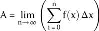
which is the exact definition of an integral, normally written in the following notation:
..................Content has been hidden....................
You can't read the all page of ebook, please click here login for view all page.