21
Thévenin’s Theorem: Circuit Analysis
21.1 Introduction
In this chapter, we will examine the Thévenin’s theorem, also known as equivalent circuit theorem, created by Léon Charles Thévenin, a French telegraph engineer who extended Ohm's law to the analysis of complex electrical circuits.
This theorem makes it possible to convert complex circuits into simpler ones that are electrically equivalent and behave in the same way.
21.2 The Theorem
Unlike the source transformation theorem, which aims to replace parts of circuits to convert everything into a voltage or current source with resistors, the Thévenin Theorem's objective is to replace the whole circuit with a voltage source in series with a resistor.
Figure 21.1 shows the goal of the Thévenin's theorem to replace a complete circuit with a voltage source, called the equivalent Thévenin voltage source, or VTh in series with a resistor, called the equivalent Thévenin resistor, or RTh.

Figure 21.1 Thévenin equivalent circuit.
21.2.1 The Equivalent Thévenin Circuit
The Thévenin circuit always represents the equivalent seen through two terminals of the original circuit that can be the input, the output, or any other points.
Figure 21.2 shows a black box representing a circuit and points A and B representing the input.
Figure 21.2 Two points of a circuit.
21.2.2 Methodology
To obtain the Thévenin equivalent circuit, we must perform the following steps:
- Remove any loads that the circuit may have.
- Remove all current sources from the circuit.
- Short‐circuit all voltage sources in the circuit.
- Calculate the equivalent resistance.
- Calculate the equivalent voltage by using nodal analysis.
21.2.3 Example
Consider the circuit shown in Figure 21.3. This circuit has a few resistors, a voltage source, a current source, and an output represented by points T and U. A load, represented by RL,1 is connected to the output.

Figure 21.3 Thévenin equivalent circuit.
21.2.3.1 Thévenin Equivalent Resistance
To find the Thévenin equivalent circuit, we must follow the theorem’s rules.
The first rule is to remove all loads from the circuit.
Figure 21.4 shows the circuit with the load removed.

Figure 21.4 Circuit with the load removed.
Next, according to the rules of Thévenin, we must remove all current sources from the circuit and replace all voltage sources with short circuits, that is, a wire. The result is seen in Figure 21.5.

Figure 21.5 All sources removed.
Points X and Y represent where the current source was. There is no more current flowing across these points now.
After removing the sources, we can redraw the circuit in Figure 21.4 as shown in Figure 21.6.

Figure 21.6 Improved version.
In the new circuit, R1 and R2 are in parallel and must be replaced by an equivalent resistance equal to
The result is seen in Figure 21.7.

Figure 21.7 Thévenin equivalent circuit without the load.
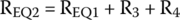
In this new circuit, we see that RE, R4, and R3 are in series and can be replaced by an equivalent resistance equal to
The result is seen in Figure 21.8.
Figure 21.8 Equivalent circuit without the sources.
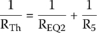
Finally, we have two resistors in parallel, RE2 and R5, and we can replace them with an equivalent resistance:
This final resistance is the Thévenin resistance.
21.2.3.2 Thévenin Equivalent Voltage
To find the Thévenin equivalent voltage, we bring back the original circuit and choose a point to use as zero reference. The result is seen in Figure 21.9.
Figure 21.9 Original circuit plus ground.
We must use nodal analysis to find the currents and the voltages across the points we have assigned in Figure 21.10.

Figure 21.10 Original Circuit plus ground with assigned currents.
21.2.3.3 Node A
By applying Kirchhoff’s current law (KCL) in the circuit shown in Figure 21.10, we get the following equation:
Every one of these currents can be described, in terms of nodal analysis, as follows:
Without the load, the current across R4 and R5 is the same, that is, i5.
Therefore,
Current i7 is the same as I1, equal to 1 A:
By substituting the values we have already discovered in (21.1), we get
21.2.3.4 Node B
The only current that flows across node B is i5. This current flows across R5 and then across R4, because there is no load connected in parallel with R5.
Therefore, we will ignore this current by now, because it is irrelevant to solve the circuit.
21.2.3.5 Node C
The current diagram has a visualization problem that makes difficult to analyze the currents of node C. The problem is the current source I1.
To best understand the circuit, we invert the position of R3 and I4 and redraw the circuit like shown in Figure 21.11.

Figure 21.11 Original circuit redrawn.
After redrawing the circuit, we see that current i6 was not really a current, it was only an illusion created by a drawing that was making it difficult to visualize the real currents in the circuit.
If we now apply KCL to node C, we get
By applying nodal analysis to the node, we get each of these currents:
21.2.3.5.1 Putting It All Back Together
We end with two equations, (21.2) and (21.4), which can be solved by using matrices

like we have described before.
The solution gives us the following result.
21.2.3.6 The Thévenin Voltage
The Thévenin voltage will be the subtraction between the voltage across A and B, or
This will be the voltage across R5.
To find this voltage we need to know the current flowing across this resistor.
In the first part of this solution, we discovered that
Therefore, the voltage across R5 is
![]() is exactly the Thévenin voltage.
is exactly the Thévenin voltage.
Now that we have the Thévenin voltage and resistance, we can redraw the final Thévenin equivalent circuit, as shown in Figure 21.12, with the load reconnected.

Figure 21.12 Thévenin equivalent circuit.
21.2.3.7 Same Behavior
In this section we will check if the Thévenin circuit behaves like the original.
Figure 21.13 shows the original circuit with the load connected and its respective currents.

Figure 21.13 Original circuit.
The load RL and resistor R5 are in parallel, and we can substitute them by an equivalent resistor with the following resistance:
We also swap, like we did before, the positions of the current source and R3. The result is seen in Figure 21.14.
To compare this circuit with the equivalent Thévenin, we must find the current and the voltage across RE.
Figure 21.14 Improved original circuit.
21.2.3.7.1 Node A
By applying KCL at node A, we get the following equation:
By applying nodal analysis to node A, we get the following equation for every term of the previous equation:
i6 = I1, the current source:
Putting it all back together,
21.2.3.8 Node C
Node C gives the following equation by applying KCL:
We already know two terms of this equation. The other two are
Putting it all back together,
We got two equations, (21.5) and (21.6), which can be solved by using matrices

The solution, by the method we have explained before, gives us
We can now calculate ie:
To calculate the voltage across RE, we must use the first Ohm’s law
We know that ie is the current flowing across RE. However, this resistor does not exist in real life and is just a substitute for RL in parallel with R5 (see Figure 21.13).
To compare this circuit with the Thévenin equivalent, we must calculate the current flowing across the load, alone.
RL and R5 are in parallel and therefore have the same voltage across. Current across each resistor is their resistance multiplied by their current. We can express both conditions mathematically and obtain a relation between their currents, as follows:
Because both resistors are in parallel, we know that
Therefore, the load current is
21.2.3.8.1 Confirmation Using the Thévenin Equivalent
In this section we will perform the same calculation using the Thévenin equivalent circuit, shown again on Figure 21.15, to see if the values match.
Figure 21.15 Thévenin equivalent circuit used previously.
The first thing is to apply the first Ohm’s law to find the current flowing across the Thévenin circuit:
Notice that this value is the same as obtained in (21.8).
The next step is to find the voltage across RL, by applying the first Ohm’s law, again:
Once more, we see that this value is the same as obtained in (21.7).
Therefore, we conclude that the Thévenin equivalent circuit behaves exactly like the original circuit.
Exercises
- Find the Thévenin equivalent of the circuit connected to a load RL, shown in Figure 21.16.

Figure 21.16 Thévenin equivalent circuit (exercise).
Solutions
To get the Thévenin resistance, we first remove the load (Figure 21.17).
Figure 21.17 Thévenin equivalent circuit without the load.
Then, according to the Thévenin rules, we remove all current sources and replace all voltage sources with short circuits (Figure 21.18).
Figure 21.18 Equivalent circuit (exercise) without the sources.
R1 and R2 are in parallel and can be replaced by an equivalent resistance equal to (Figure 21.19)
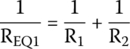


Figure 21.19 Thévenin equivalent circuit (exercise).
REQ1, R3, and R4 are in series and can be replaced by an equivalent resistance equal to the sum of their individual resistances (Figure 21.20):
Figure 21.20 Thévenin equivalent circuit (exercise).

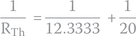
The Thévenin resistance will be the equivalent resistance of REQ2 in parallel with R5:
Thévenin Voltage
To find the Thévenin voltage, we go back to the original circuit without the load, add a zero‐reference point to it, and assign currents to all branches with directions at random as seen in Figure 21.21.

Figure 21.21 Thévenin equivalent circuit – branch currents.
To find the voltage across points A and B, we must apply KCL to all nodes.
Node C
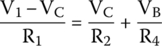
By applying KCL to node C, we get the following equation:
Nodal analysis of node C gives us the following current equations:
Putting it all back together and substituting the known values, we get


Node B
KCL gives us the following equation:
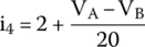
By nodal analysis, we get that
Therefore,
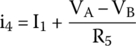
However, i4 is also

Therefore, we can equate both equations for i4 and obtain a second equation:
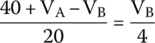

By applying KCL to the ground node we also get
Therefore, we can get a third equation by substituting the values we have so far:

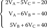
We end with three equations, (21.9), (21.10), and (21.11):
To make it simple, we take the first equation and solve for VA

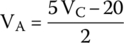
and substitute this value on the second equation:


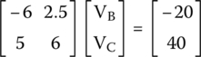
We now have two equations instead of three:

These equations can be written into the matrix form, which we already know how to solve:
The solution gives the following.
If we substitute VC in (21.12), we obtain the following.
The Thévenin voltage will be the voltage across points A and B that is equal to the difference between VA and VB, or


Note
- 1 A load can be anything, a motor, a light bulb, headphones, etc.