22
Norton’s Theorem: Circuit Analysis
22.1 Introduction
In this chapter, we will examine Norton’s theorem, also known as Mayer’s theorem, developed at the same time, in 1926, by Hans Ferdinand Mayer, researcher of Siemens & Halske in Germany, and by Edward Lawry Norton, engineer and researcher of the legendary Bell Labs1 in the United States.
22.2 Norton’s Theorem
Following the idea of Thévenin’s theorem, Norton’s theorem proposes the replacement of complex circuits with an equivalent simplified version, known as Norton equivalent circuit.
Figure 22.1 Norton equivalent circuit.
Thévenin theorem replaces the original circuit with a voltage source in series with a resistor. Norton’s theorem, however, replaces the original circuit with a current source in parallel with a resistor, like shown in Figure 22.1.
22.2.1 Finding Norton Equivalent Circuit
Like Thévenin, Norton equivalent circuit is always equivalent to two chosen points in a circuit, like the input, the output, etc. Different points in a circuit will generate different Norton circuits.
22.2.2 Methodology
These rules must be followed to obtain the Norton equivalent circuit:
- Create a new circuit version where the load is short‐circuited, and calculate the current source using nodal analysis and Kirchhoff’s current law (KCL).
- Create a new circuit version without the load, without all current sources, and with all voltage sources replaced with short circuits, and find the equivalent resistance.
22.2.3 Example
Find Norton equivalent circuit for the one shown in Figure 22.2.
Figure 22.2 Original circuit.
This circuit is the same as used in the last chapter, composed of several resistors, two sources, and a load represented by RL.
22.2.3.1 Finding the Norton Current Source
To find the Norton current source, that is, the current flowing between points A and B, without the load, we follow the rules defined by Norton. The first one is to replace the load with a short circuit.
The result is seen in Figure 22.3.
Figure 22.3 Load is short‐circuited.
Replacing the load with a short circuit also short‐circuited R5 that can now be removed from the circuit.
The result is seen in Figure 22.4.

Figure 22.4 Original circuit.
The Norton current for this circuit is the one flowing between points A and B, without the load. In the given example, the Norton current will be equal to i4, in the circuit seen in Figure 22.5.
Figure 22.5 Norton current.
To find the Norton current, we must analyze all circuit nodes.
22.2.3.1.1 Node A
By applying KCL on node A, we get
The other unknowns of this equation are
Putting it all back together,
22.2.3.1.2 Node C
KCL on node C gives us the following equation:
We have that
Putting it all back together,
We end with two equations, (22.1) and (22.2):
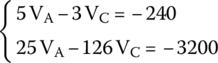
We can solve this system of simultaneous equations by using matrices and by using the method we already explained:
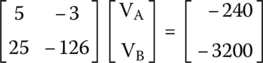
The solution gives VA and VC:
We can now find the Norton current
The negative sign for i4 shows that this current, in fact, flows in a direction opposite to the one we have arbitrarily chosen.
22.2.3.1.3 Norton Equivalent Resistance
In this next phase of the Norton theorem, we must find the Norton equivalent resistance.
The method used to find this value is the same used by the Thévenin method. Because this circuit is the same as used in the Thévenin chapter of this book, we already know the resistance value, that is, equal to the following value.
Therefore, the Norton equivalent circuit will have the final form shown in Figure 22.6.

Figure 22.6 Final Norton equivalent circuit.
22.2.3.1.4 Confirmation
In the last chapter we have confirmed that the Thévenin Equivalent Circuit was electrically equivalent to the original circuit.
In this chapter we are using the same circuit as before. If we confirm that this Norton equivalent circuit is the same as the Thévenin equivalent circuit calculated in the last chapter, we know that we have the right values.
To do that, we must use the knowledge we have already acquired about source transformations and convert this Norton equivalent circuit, that is, nothing more than a current source in parallel with a resistor, into a voltage source in series with the same resistor that is equivalent to the Thévenin circuit.
To convert the current source in parallel with a resistor into a voltage source in series with the same resistor, we know that the voltage source can be found by using the following formula:
This is the same value found in the last chapter for the voltage source. We conclude that this circuit was calculated correctly.
Exercises
- Find the Norton equivalent circuit for the circuit shown in Figure 22.7.
Figure 22.7 Finding the Norton equivalent circuit (exercise).
Solutions
Following Norton rules, we replace the load with a short circuit (Figure 22.8).

Figure 22.8 Load replaced with a short circuit.
Resistor R5 was bypassed by the short circuit and can be removed from the circuit (Figure 22.9).
Figure 22.9 Load replaced with a short circuit.
We must apply nodal analysis to node A to find currents i1 and i2.
Node A
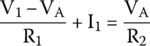
By applying nodal analysis to node A, we get the following equations:
KCL on node A gives us the next equation:
Therefore,
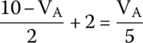
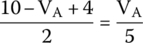


Using this value, we can calculate the currents

Interestingly, we see that i1 is 0! Therefore, there is no current flowing in the branch formed by V1 and R1. Current is just flowing in the other half of the circuit (Figure 22.10).
We conclude that current i4 is then equal to I1 and equivalent to the Norton current.
Figure 22.10 Final Norton equivalent circuit.
Norton Equivalent Resistance
To find the Norton equivalent resistance, we must use the same method used in the Thévenin method.
Therefore, we bring back the original circuit with the load removed (Figure 22.11).
Figure 22.11 Norton equivalent circuit.
To find the Norton equivalent resistance, that is, the resistance between point A and ground, we remove all current sources and replace all voltage sources with short circuits (Figure 22.12).
Figure 22.12 Norton equivalent circuit.
We see that the left part of the circuit is not connected to the right part anymore and can be removed from the circuit. We also see that the left side of R4 is not connected to anything and can also be removed.
The only thing remaining between A and ground is R2 and this is the Norton resistance.
Therefore, the Norton equivalent circuit is equal to the one shown in Figure 22.13.
Figure 22.13 Final Norton equivalent circuit.
Note
- 1 Famous research and development laboratory created in 1870 by Bell Telephone System, company originally founded by Alexander Graham Bell. Researchers working at Bell Labs, awarded with nine Nobel Prizes, are credited with the development of the transistor, LASER, CCDs used in digital photography, radio astronomy, first satellite, photo cell, mobile telephony, and UNIX operating system, including programming languages like C and C++, contributing immensely to the modern society we live today.