27
RLC Circuits: Part 1: Voltage Analysis in Circuits Containing Resistors, Capacitors, and Inductors in Series
27.1 Introduction
Previously in this book, we have examined RC and RL series circuits and how capacitors and inductors react when subjected to voltage or current changes.
We saw that capacitors and inductors can store potential energy in the form of electric or magnetic fields.
RC and RL circuits are circuits that contain one element that can store energy, and for that reason, all equations we have found are first‐order differential equations.
However, RLC circuits contain two elements that can store energy, and at this point, the readers have realized that these circuits will produce second‐order differential equations.
Due to the complexity of this theme, we will divide the analysis of RLC series circuits into two parts. In this chapter we will make a voltage analysis and in the next chapter a current analysis.
27.2 A Basic RLC Series Circuit
Figure 27.1 shows a circuit with a voltage source, a switch, a resistor, an inductor, and a capacitor in series.
Figure 27.1 A basic RLC circuit.
The switch is open, there is no current flowing in the circuit, the inductor is completely de‐energized, and the capacitor is completely discharged.
At time t = 0 s, the switch is closed, and current flows and reaches the inductor.
The current that was zero before has now a nonzero value. The inductor hates this current variation and tries to block its flow by generating an opposite electromotive force. This electromotive force manifests itself by making a voltage rise across the inductor with the same value as the power supply but with the inverted polarity.
Therefore, current does not reach the capacitor at this first moment, and the inductor is seen, by the circuit, as an open circuit or a resistor with infinite resistance.
As time passes, current starts to flow through the inductor and reaches the capacitor. Initially the capacitor is completely discharged and will behave like a short circuit, letting all current flow without any resistance. Voltage across the capacitor is 0.
Time passes and the inductor starts to store energy in the form of magnetic field and, at the same time, the capacitor is charging.
As the capacitor reaches its maximum charge, it starts to prevent current from flowing by generating an electromotive force that starts to reduce current gradually.
The inductor sees this current reduction and is trying to prevent that to happen; by using the energy, it has stored in the form of magnetic field to create an electromotive force to push current forward and keep it flowing.
What happens now depends on the values of the capacitor and the inductor, as we will see in the following chapters of this book, but one option is that the inductor will try to force the current to keep flowing against the capacitor’s will.
The process will remove charges from the capacitor’s plate that was already filled with charges to the other, forcing this component to begin charging with the opposite polarity.
When the capacitor’s charge reaches the point where its force is bigger than the inductor’s force, the process will reverse: the capacitor will start to discharge through the inductor, forcing current on the opposite direction, and that current will energize the inductor.
The cycle repeats, with one component transferring energy to the other until all energy is gone.
This energy exchange is seen as an oscillation.
The kind of oscillation we just described can be illustrated in terms of voltage variations across the capacitor by the graphics in Figure 27.2. Notice that the voltage oscillates around the power supply voltage V1, which will be the final capacitor’s voltage.
Figure 27.2 A basic RLC circuit.
Notice that the voltage rises above the power supply value and oscillates around before stabilizing.
The voltage decays or rises exponentially and has a direct relation to the values of capacitance and inductance, as we will see forward in this book.
The frequency the oscillations happen is called the angular frequency or resonant frequency, also known as the natural resonant frequency, and can be found by the following formula.
Because the angular frequency is related to the frequency by
we can find the circuit’s oscillation frequency by using the following formula.
As the oscillations happen, they are damped. The much they are dumped are ruled by the dumping factor, calculated by the following formula.
27.2.1 Circuit Analysis
To understand what happens on a series RLC circuit, we must examine the circuit behavior in terms of voltage across the capacitor.
The circuit is the one shown in Figure 27.1 that we repeat again in Figure 27.3 for convenience.

Figure 27.3 A basic RLC circuit.
The switch is open, there is no current flowing in the circuit, the inductor is completely de‐energized, and the capacitor is completely discharged.
At time t = 0 s, the switch is closed, and current flows and reaches the inductor.
27.2.2 Voltage Across the Capacitor
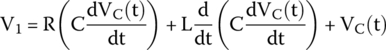
If we analyze a series RLC circuit, we get that the power supply voltage is equal to the sum of the voltage drop across the resistor, the voltage across the inductor, and the voltage across the capacitor, or mathematically
We know the voltage across the inductor is
and the voltage drop across the resistor is
Therefore, the previous equation changes to
However, we also know that the current across the capacitor is defined as
and that this current, in the example of an RLC circuit in series, is the same current that flows across the circuit.
Therefore, we can substitute i(t) in (27.3) and obtain

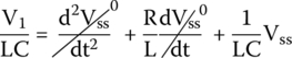
We divide everything by LC to write the equation using the standard form as
We see, by the squared term in the Eq. (27.4), that this is a second‐order differential equation, like we have predicted before.
To solve this equation, we must have a few mathematical concepts in mind.
27.2.3 Back to the Equation
Applying this mathematical concept for the series RLC circuit, we see that the voltage across the capacitor will have two equations: one representing the transient state and another representing the steady state, or
27.2.3.1 Steady‐State Solution
After an infinite time has passed, the voltage across the capacitor will stabilize in a value that we know will be the same as the power supply voltage, but, to confirm this fact, let us work with the equations.
To solve the differential equation in (27.4) for the steady‐state solution, consider that
Therefore, the Eq. (27.4) can be written as
We know that Vss is a constant value, because this voltage is equal to the constant power supply voltage. Therefore, we can apply the following concept.
We can simplify the equation
This result shows that Vss will be equal to V1, as expected.
27.2.4 Transient Solution
To find the transient solution, we must solve the equation that represents that state, described as follows:
This equation can be written in a simplified way:
which is a homogeneous differential equation with constant coefficients.
To understand how to solve this kind of equation, we must understand the following mathematical concept.
By applying this mathematical concept, we see that the equation to be adopted as a solution will have the generic form:
By adapting this equation for the given example, we get the transient voltage equation having the form
Therefore, we can convert the equation into
We see a lot of terms that are derivatives of exponentials and we can apply the following concept.
Therefore, the terms and their results are
and
Therefore, by substituting these terms, we get
Looking at this equation, we see that it is formed by two parts,

and that the whole equation is equal to 0. For this to be true, one of the parts (1 or 2) must be 0.
For the second term to be 0, or
the term m will have to be equal to −∞. If this is true, we get
We end with A = 0, a situation that does not bring any useful solution for our equations.
Therefore, the first part must be the one equal to 0, or
27.2.4.1 The Roots of the Equation
The previous equation is a quadratic equation and we know how to solve that and obtain the roots of the equation by using the formula
Therefore,

or we can rewrite it as

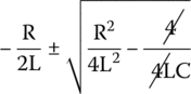
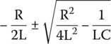
We can simplify this equation by substituting the values inside the radical with those of the angular frequency and damping defined before:
And we get the roots of the equation.
Consequently, the roots defined by (27.5) will be two:
Looking at the term inside the radical, we see that we can have basically three kinds of results, depending on the term ![]() , be positive, negative, or 0.
, be positive, negative, or 0.
In the next sections, we will examine each case.
27.2.4.2 Critically Damped Solution
This is the case where α = ω0, or the damping factor is equal to the angular frequency and the result of ![]() , inside the radical, is 0.
, inside the radical, is 0.
This case will give us just one root for the equation, which will be a negative number, as follows:
We know that the complete solution for the equation for voltage across the capacitor will be the sum of the transient solution with the steady‐state solution, or
We also know that the voltage across the capacitor when the circuit reaches the steady state will be the same as the power supply voltage, V1.
Another thing we know is that the final equation for the transient solution must contain two terms in the form of y = Aemt, something like
However, we see that the critically damped solution has only one root m = − α, which will lead to a transient solution containing only one term, like
This equation does not represent the truth. The real equation must contain two terms because the circuit has two initial conditions that must be taken into consideration: the initial voltage across the capacitor and the initial current flowing in the circuit the moment the switch is closed.
We must discard this equation and find a way to discover the correct one.
27.2.4.2.1 Going Back to the Original Equation
We know that
Therefore,
We also know that
Thus,
If we substitute the condition of the critically damped solution, ω0 = α, in (27.8), we get
If we now substitute (27.7) and (27.9) in (27.6), we obtain
We can rewrite this equation as
To simplify, let us create a new variable y:
We can use this variable in (27.10) and simplify that equation to
Like we have examined before, the solution for the Eq. (27.11) is known to be
Therefore, we can convert Eq. (27.11) into
We can manipulate this equation to get A:
It may not appear now but the Eq. (27.13) is equal to the following derivative:
due to the product rule from calculus.
The following is the mathematical concept.
By applying this rule, the derivative
will be equal to
which is equal to
Compare (27.13) with (27.14). They are the same equation. See how in (27.13) the second term coefficient is equal to α and in (27.14) the same coefficient is equal to −m, which is perfectly true because m = − α, as we have calculated before.
Therefore, Eq. (27.13) can be converted into
If we integrate both sides of this equation with respect to time, we get
That gives us
Constants C1 and C2 can be combined and replaced by a single constant B.
Consequently, the equation simplifies to
We can manipulate this equation to find Vtr(t):
or
We can substitute m with −α and get the final transient equation:
Therefore, the final equation for the voltage across the capacitor considering the transient and the steady‐state solutions is equal to the following equation.
To find the values of A and B, we must use the circuit’s initial conditions.
27.2.4.2.2 First Condition (VC(0))
The first condition to consider in the series RLC circuit is the voltage across the capacitor at time t = 0 s. We call this voltage V0.
To obtain the first constant, we take Eq. (27.15) and solve it for t = 0 s:
27.2.4.2.3 Second Condition (dVC(0)/dt)
The second condition we must consider is the current flowing in the circuit at time t = 0 s.
Current on a capacitor is defined as the derivative of voltage with respect to time, or
Therefore, all we must do to get the current equation is to find the derivative of the voltage equation (27.15) with respect to time, find the current equation, and solve this other equation for t = 0s.
Thus, we take the equation
and take the derivative
The first term
is equivalent to the current across the capacitor.
To solve this first term, we must consider the following.
We have no means to guarantee that the current across the capacitor will be 0 at time 0 by examining the capacitor alone. Capacitors resist changes in voltages but not in current. However, the capacitor is in series with an inductor and inductors resist current changes. We can, therefore, guarantee that current at time 0 will be 0, and we can simplify (27.17) to

The last term is the derivative of a constant.
Therefore,
To solve the first term
we use the following math concept.
that gives us this

producing this solution:
The second term of Eq. (27.18)
is a simple derivative of an exponential, for which we have the following math concept.
that gives the following result:
Putting (27.19) and (27.20) back into (27.18),
Solving for t = 0
−αAte−αt + Ae−αt − αBe−αt = 0
−αAt + A − αB = 0
which gives us
But B was obtained in (27.16) as
Consequently, A is
27.2.4.2.4 Voltage Curve
The critically damped circuit will not have an oscillatory behavior because the damping coefficient will prevent that from happening.
Figure 27.4 Voltage across the capacitor (critically damped solution).
Figure 27.4 shows the curve for the total solution for the voltage across the capacitor for a critically damped series RLC circuit. Notice how the curve starts at 0 and increases exponentially until it stabilizes at a voltage equal to the power supply (V1).
27.2.4.3 Overdamped Solution
This is the case where α > ω0, or the damping coefficient is greater than the angular frequency and the result of ![]() , inside the radical, is positive.
, inside the radical, is positive.
Therefore, the roots m1 and m2 will be different, negative, and real numbers as follows:
Like the critically damped solution, the overdamped solution will not present an oscillatory behavior.
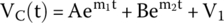
Because the equation has two distinct solutions and we know that the solution for the transient phase respects the form y = Aemt, we conclude that the transient equation for the voltage across the capacitor during the transient phase must have two terms according to the form
Therefore, the total solution for the voltage across the capacitor must include the voltage across the capacitor during the steady‐state phase, which we know to be the same as the power supply V1.
To find the values of A and B, we must use the circuit’s initial conditions.
27.2.4.3.1 First Condition (VC(0))
The first condition to consider in the series RLC circuit is the voltage across the capacitor at time t = 0 s. We call this voltage V0.
To obtain the first constant, we take Eq. (27.21) and solve it for t = 0 s:
27.2.4.3.2 Second Condition (dVC(0)/dt)
The second condition we must consider is the current flowing in the circuit at time t = 0 s.
Like before, current on a capacitor is defined as the derivative of voltage with respect to time, or
Therefore, all we must do to get the current equation is to find the derivative of the voltage equation (27.21) with respect to time:
The first and the last terms are 0 for the same reason explained on the critically damped solution, because the initial current is 0 and because the derivative of a constant is 0.
Therefore,
At this point we already know how to solve the derivative of an exponential.
Thus, the solution for the previous derivatives is
Solving this equation for t = 0 s,
We end with two equations, (27.22) and (27.23):

From the first equation we get A:
By substituting this value on the second equation, we obtain
Upon substituting B in (27.22), we get

and we will obtain the following formula.
27.2.4.3.3 Voltage Curve
The overdamped circuit will not have an oscillatory behavior because the damping coefficient will prevent that from happening after a few brief oscillations.

Figure 27.5 Voltage across the capacitor (overdamped solution).
Figure 27.5 shows the curve for the voltage across the capacitor. Notice how the curve grows exponentially and stabilizes in a value greater than the power supply voltage V1.
27.2.4.4 Underdamped Solution
This is the case where α < ω0, or the damping coefficient is smaller than the angular frequency and the result of ![]() , inside the radical, is negative.
, inside the radical, is negative.
This case will give us two roots that are complex numbers as follows:
The equations can be simplified by defining
Therefore, the roots will have the form
Like before, we know that the solution for this equation follows the form y = Aemt and will have the following form for two distinct roots, as defined before in this book:
Upon substituting m1 and m2 in this equation, we get
Therefore,
Several terms of Eq. (27.24) are complex exponentials. Fortunately, there is a mathematical definition created by Euler that relates complex exponentials with sines and cosines, which will provide a way to convert equation (27.24) to a friendlier form.
The following is what the definition says.
By applying this concept, we can convert equation (27.24) into
and we get the final formula for the voltage across the capacitor for the underdamped solution.
Again, to find K1 and K2, we must apply the circuit’s initial conditions, like we did on the previous cases.
27.2.4.4.1 First Condition (VC(0))
The first condition to consider in the series RLC circuit is the voltage across the capacitor at time t = 0 s. We call this voltage V0.
To obtain the first constant we take Eq. (27.25) and solve it for t = 0 s:
We get the first constant of Eq. (27.25):
27.2.4.4.2 Second Condition (dVC(0)/dt)
The second condition we must consider is the current flowing in the circuit at time t = 0 s.
Current on a capacitor is defined as the derivative of voltage with respect to time, or
Therefore, all we must do to obtain the current equation is to find the derivative of the voltage equation (27.25) with respect to time.
Therefore, we take the voltage equation
and take the derivative
and rewrite
To make it easy, let us expand the equation by using the following concept.
Thus, we can expand the equation
Rearranging
Observe Eq. (27.27) in the illustrated form below:
This equation shows that we are before two derivatives of a product of two functions, u and v, and that we can apply the following math concept to solve both derivatives.
This will expand Eq. (27.28) into
Equation (27.29) can be divided into four parts, namely A, B, C, and D. We will solve these parts independently to make it easy.
27.2.4.4.2.1 Solving Parts A and C
Parts A and C are equal. They are both derivatives of an exponential and we already know how to solve them.
Parts A and C will produce the following result:
27.2.4.4.2.2 Solving Part B
To solve part B, we will need a new math concept shown below.
By applying this concept, we get the following result for part B:
27.2.4.4.2.3 Solving Part D
To solve part D, we will need another new math concept.
By applying this rule, we get the following result for part D:
By putting (27.30), (27.31), and (27.32) back into (27.29), we get
Solving for t = 0 s, we get
But as defined by (27.26),
Therefore, we get the second constant of Eq. (27.25):
Figure 27.6 Voltage across the capacitor (underdamped solution).
27.2.4.4.3 Voltage Curve
The underdamped circuit will present an oscillatory behavior.
Figure 27.6 shows the curve for the voltage across the capacitor. Notice how the voltage oscillates up and down until it stabilizes at the same value as the power supply V1.
27.3 Examples
27.3.1 Example 1
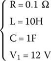
Figure 27.7 shows a circuit with a direct voltage source, a switch, a resistor, an inductor, and a capacitor in series.
The switch is open, there is no current flowing in the circuit, the inductor is completely de‐energized, and the capacitor is completely discharged.
At time t = 0 s, the switch is closed, and current flows and reaches the inductor.
The following is what we want to find about the circuit:
- What is the voltage across the capacitor after the switch is closed?
- What is the voltage across the capacitor 2 sec after the switch is closed?
- What is the circuit’s natural resonance frequency?
Figure 27.7 DC powered series RLC circuit.
27.3.1.1 What Is the Voltage Across the Capacitor After the Switch Is Closed?
When the switch is closed, current flows and reaches the inductor. The inductor hates sudden variations of current and will prevent current from flowing as soon as the switch is closed.
Therefore, there is no current reaching the capacitor, which is initially discharged, and the voltage across the capacitor is 0.
27.3.1.2 What Is the Voltage Across the Capacitor Two Seconds After the Switch Is Closed?
We can have three kinds of series RLC circuits, namely, critically damped, overdamped, and underdamped, each one with its own equations for the voltage across the capacitor.
The first thing we need to do is to know which circuit is this one.
The given values are
We first calculate α and ωo:
We see that α < ω0, equivalent to an underdamped circuit.
The equation for the voltage across the capacitor, for this case, is
In the following steps, we will find the several unknowns in the previous equation:
This is the square root of a negative number. We must remember this math concept from the imaginary numbers.
Therefore,
can be written as
extracting the root of the imaginary part:
or
which results into
The capacitor is initially discharged; therefore, V0 is 0. The power supply voltage, V1, is equal to 12 V.
Therefore, we can find K1,
and K2,
Now that we have all unknowns, the complete formula for the voltage across the capacitor can be assembled like this:
Finding the voltage for t = 2 s,
27.3.1.3 What Is the Circuit’s Natural Resonance Frequency?
The natural resonance frequency for the series RLC circuit is given by the following formula:
This low value for the frequency was expected due to the high values of capacitance and inductance. Big capacitors and inductors are slow to respond to changes, for example, a transatlantic boat is slow compared with a race boat in the agility to do fast curves and start/stop moving.
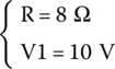
27.3.2 Example 2
Consider the same circuit as the previous example. The values of L and C are unknown, but R and V1 are
Like in the previous circuit, the switch is open.
At time t = 0 s, the switch is closed, and current flows and reaches the inductor.
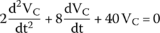
The circuit is ruled by the following second‐order differential equation:
The initial conditions for the circuit are as follows: the voltage across the capacitor for t = 0 s is 2 V, and the first derivative of the voltage equation with respect to time, for t = 0 s, is equal to 4 A.
Mathematically speaking,
The following is what we want to find about the circuit:
- The complete equation for the voltage across the capacitor.
- The voltage across the capacitor for t = 2 s.
27.3.2.1 The Complete Equation for the Voltage Across the Capacitor
The second‐order differential equation for a series RLC circuit follows the form
which we repeat as follows:

If we compare A and B of this equation with the same values of Eq. (27.34), which we repeat in the following,

we can extract a lot of elements, for example,
In this given example,
By substituting R in (27.36), we get
Another part we can extract by comparing equation (27.34) with (27.35) is
The inductor is
Therefore, by substituting L in (27.37), we get
Equation (27.34) can be written in a simplified form as
This is a quadratic equation and its roots can be found by using the classical formula:
The equation has only one root, which is typical of a critically damped circuit, governed by an equation for the voltage across the capacitor that follows the form
First, we need to find α:
To find the coefficients A and B in Eq. (27.38), we must apply the circuit’s initial conditions.
The first condition is the initial voltage across the capacitor for time 0. This is a given condition defined as
Therefore, we take the original equation
and solve it for t = 0 s to find the first coefficient:
For time t = 0 s,
To find the second coefficient, we must apply the circuit’s second condition and solve the equation for t = 0 s. This is also a condition provided by the example definition:
Therefore, we take the original equation (27.38)
and take the derivative with respect to time:
The first term, as defined by the problem, is
The last term
is a derivative of a constant and that is mathematically 0.
The middle term is a derivative of a product of two functions, or
which can be solved by applying the following concept.
Therefore, the original equation can be expanded into
and solved as
Upon substituting the known values
and solving for t = 0 s to get the other coefficient,
Therefore, the final equation for the voltage across the capacitor is shown as follows.
Calculating the voltage across the capacitor for t = 2 s,
Exercises
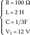
- Consider the circuit shown in Figure 27.8, composed of a resistor, an inductor, a capacitor, a direct voltage power supply, and a switch.

Figure 27.8 DC powered series RLC circuit.
The switch is initially open, the capacitor is completely discharged, and the inductor is completely de‐energized.
These are the components:
At time t = 0 s, the switch is closed, and current flows and reaches the inductor.
The following is what we want to find about the circuit:
- What is the voltage across the capacitor as soon as the switch is closed?
- What is the complete equation for the voltage across the capacitor?
- What is the voltage across the capacitor 5 s after the switch is closed?
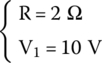
- Consider a series RLC circuit like the previous one. The values of all components are the same, except R and V1, as shown next:
The circuit is ruled by the following second‐order differential equation:
This circuit’s initial conditions are
The following is what we want to find about the circuit:
- The complete equation for the voltage across the capacitor.
- The voltage across the capacitor for t = 3 s.
Solutions
What is the voltage across the capacitor after the switch is closed?
After the switch is closed, current flows and reaches the inductor. The inductor hates sudden current variations and will not let this new current pass.
Therefore, no current reaches the capacitor, which is continuously discharged.
What is the complete equation for the voltage across the capacitor?
We can have three kinds of series RLC circuits, namely, critically damped, overdamped, and underdamped, each one with its own equations for the voltage across the capacitor.
The first thing we need to do is to know which circuit is this one.
The given values are

We first calculate α and ωo:


We see that α > ω0, equivalent to an overdamped circuit.
The equation for the voltage across the capacitor, for this case, is
The roots of an overdamped solution are
and
The coefficients in Eq. (27.37) are


and


Having found all unknowns, we can write the final equation for the voltage across the capacitor (27.39) as
What is the voltage across the capacitor 5s after the switch is closed?
We use the last equation and solve for t = 5 s:

- The complete equation for the voltage across the capacitor.
The given circuit is ruled by the following equation:
We divide the equation by 2 to write it in the standard form as
Series RLC circuits are ruled by the following second‐order differential equation:
which we rewrite as follows:

If we compare A and B of this equation with the same values of Eq. (27.40), which we rewrite in the following,
(27.41)
we can extract several values:
In this given example,

By substituting R in (27.42), we get
Another part we can extract by comparing the equations is
Therefore, by substituting L in (27.43), we get
The next thing we must do is to find if this is a critically damped, overdamped, or underdamped circuit.
We proceed to calculate α


and ω0

We see that α < ω0. Therefore, this is an underdamped series RLC circuit, ruled by the following equation for the voltage across the capacitor:
We proceed finding the unknowns: first K1


and then K2

To find K2 we need to find ωd:

Therefore,

The complete equation for the voltage across the capacitor can be assembled as follows.
The voltage across the capacitor for t = 3 s.
Using the last equation, we can solve for t = 3 s:

