23
Superposition Theorem: Circuit Analysis
23.1 Introduction
In this chapter, we will examine the superposition theorem, another technique for circuit analysis.
23.2 The Theorem
The superposition theorem states that a circuit with multiple voltage and current sources is equal to the sum of simplified circuits using just one of the sources.
A circuit composed of two voltage sources, for example, will be equal to the sum of two circuits, each one using one of the sources and having the other removed.
23.3 Methodology
To simplify a circuit using the superposition theorem, the following steps must be followed:
- Identify all current and voltage sources in the circuit.
- Create multiple versions of the circuit, every version containing just one of the sources. The other sources must be removed using the following rule: voltage sources must be replaced with a short circuit and current sources just removed from the circuit.
- Find the currents and voltages required.
- Sum the results obtained in all circuits.
23.4 Example
Consider the circuit shown in Figure 23.1, which we have used in the previous chapters. We want to find the current flowing across R3 and the voltage across points A and B.

Figure 23.1 Circuit for superposition analysis.
Following the rules of superposition, this circuit will be equal to a first one containing just the voltage source V1 plus a second one containing just the current source I1.
23.4.1 First Circuit
To create the first circuit, we remove the load (RL) and the current source from the original circuit and keep just the voltage source. The result is shown in Figure 23.2.
Figure 23.2 First circuit for superposition analysis.
Next, we will perform a nodal analysis.
23.4.1.1 Node C
By applying Kirchhoff’s current law (KCL) to node C, we get the following equation:
Every term of this equation can be discovered by performing a nodal analysis to node C:
Putting it all back together,
23.4.1.2 Relation Between Voltage A and C
By observing Figure 23.2, it is clear that current i3 that was defined previously as
can also be defined as
Therefore, we can equate both equations and get VC:
By substituting this value in (23.1), we get
and we now can find VC:
Therefore, the current i3 for the first superposition circuit will be
23.4.1.3 Voltage B
Voltage across B is easy to find by simply applying the first Ohm’s law
We already have VA and we now need to find VAB that we know is equal to VA subtracted from VB.
Therefore,
and we get VAB for the first superposition circuit.
23.4.2 Second Circuit
In this section we analyze and build the second superposition circuit.
For this circuit, we must replace the voltage source, in the given example V1, with a short circuit and keep the current source.
The result is shown in Figure 23.3.

Figure 23.3 Second circuit for superposition analysis.
Replacing V1 with a wire, put R1 and R2 in parallel, and we can substitute them with an equivalent resistor:
The result is shown in Figure 23.4.
It is now time to perform a nodal analysis.
23.4.2.1 Node A
By applying KCL to node A, we get the following equation:
Figure 23.4 Second circuit for superposition analysis simplified.
By nodal analysis, we get the unknown terms of this equation:
Putting it all back together,
23.4.2.2 Node C
By applying KCL to node C, we get the following equation:
By nodal analysis, we get the unknown terms of this equation:
Putting it all back together,
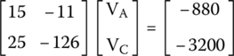
We get two equations, (23.2) and (23.3), which we can solve by using the matrix method we already know:

The solution of this simultaneous equation system will be
Finding the currents,
The current we want, i3, for the second superposition circuit is equal to
We can know calculate VB:
We know that the voltage across A and B for the second superposition circuit is equal to
23.4.2.3 Final Result
In the first superposition circuit, we have found values for VAB and i3 equal to 3.715 V and 0.03715A , respectively.
In the second superposition circuit, the values for VAB and i3 found were −25.0156 V and 0.7499 A, respectively.
By following the superposition theorem rules, we must now sum both results to get the final result.
Therefore,
and current i3
23.4.3 Checking
To confirm the results we have gotten so far, we will perform a nodal analysis of the original circuit without the load, which is shown in Figure 23.5.

Figure 23.5 Checking.
23.4.3.1 Node A
By applying KCL to node A, we get
The unknown terms of this equation are found by nodal analysis:
Putting it all back together,
23.4.3.2 Node C
KCL gives us the following equation for node C:
The unknown terms of these equations are found by nodal analysis:
Putting it all back together,
We get Eqs. (23.4) and (23.5) that can be solved using matrices
The result is
23.4.3.3 Voltage Across A and B
Now that we have VA and VC, we can calculate i3:
To find the voltage across A and B, we first need to calculate i4:
Therefore,
It is now easy to find the voltage across A and B:
The results we have found are the same as we got in previous chapters, confirming that the superposition theory describes precisely the circuit.
Exercises
- Consider the circuit shown in Figure 23.6. Find the current flowing across R2 and the voltage across A and B.

Figure 23.6 Superposition theorem (exercise).
Solutions
First Circuit
The first thing to do is to remove all current sources, from the circuit, and keep just the voltage source. The result is shown in Figure 23.7.

Figure 23.7 Superposition – first circuit (exercise).
All currents have disappeared now, except for i1 that is equal to


Voltage across A and B can be found by the first Ohm’s law


Second Circuit
To create the second circuit, we keep current source I2, remove current source I1, and short‐circuit voltage source V1. The resulting circuit is shown in Figure 23.8.

Figure 23.8 Superposition – second circuit (exercise).
To simplify the equations we can invert the direction of i2. See Figure 23.9.

Figure 23.9 Superposition – second circuit simplified (exercise).
The sum of currents, i1 and i2, is equal to current source I2.

The branch on the left, equivalent to resistor R1, is 20 Ω and the branch in the right, equivalent to the sum of R2 and R3, is 15 Ω. If we divide the resistance of the right branch by the left branch, we obtain a relation between them equal to 0.75 or, in other words, 75%. If the resistance of the right branch is 75% of the resistance of the left branch, the current of the left branch, i1, will be 75% of the current of the right branch, i2.

If

then,
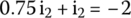

Consequently,


Third Circuit
To create the third circuit, we keep current source I2 and remove current source I1 and short‐circuit voltage source V1.
As in the last circuit, the directions of i1 and i3 can be inferred by the direction of I1. The resulting circuit is shown in Figure 23.10.
The sum of resistors R1 and R3 is parallel with R2. The equivalent resistance of this block is equal
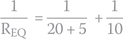
Therefore, VA will be


Thus current i3 is


Consequently, we can now calculate the voltage across A and B.


Final Result
Now that we have found all three superposition circuits, it is time to sum the results of each superposition circuit.
Therefore,


