![]()
10
Inductors: Temperamental Devices
10.1 Introduction
In this chapter, we will examine an important kind of passive component called inductor, also known as solenoid, coil, or choke.
10.2 The Inductor
It is known that a current flowing in a wire creates a magnetic field, but what happens to the magnetic field when the wire is wounded to a coil, like the one shown in Figure 10.1? Is the field the same as if the wire was straight?

Figure 10.1 Wire wounded to a coil.
No, the field is not the same. The winding creates a single longitudinal magnetic field that is the combination of all magnetic fields of the coil sections.
In Figure 10.2, the arrow shows the magnetic field created by a coil for a current that enters by the base.

Figure 10.2 Magnetic field generated by a coil for the current entering its base.
The magnetic field generated by a coil is basically located inside the coil.
Magnetic fields are measured in Tesla and represented by the uppercase letter T in the SI.
Figure 10.3 shows a transversal section of an inductor like the one shown in Figure 10.2 and its respective magnetic field lines. Figure 10.3 also shows how each of the individual magnetic field lines combines to generate a stronger longitudinal magnetic field (B).
Figure 10.3 Magnetic field in a coil transversal section.
Figure 10.4 shows the symbol used to represent inductors on schematics and in literature in general.

Figure 10.4 Inductor symbol.
10.3 Coils and Magnets
When a magnetic field is created by a coil, it makes the coil a kind of magnet.
In the examples we have given so far, coils were created by winding wires alone in air. But if the coil nucleus is a ferromagnetic rod instead of air, these rods will become magnets when current flows.
Ferromagnetic materials will have their atoms aligned by the magnetic field generated by the coil and behave like real magnets. Therefore, we can create magnets that can be turned on and off.
An invention was born: the electromagnet.
10.4 Inductance
Like we have examined before, capacitors store potential energy in the form of electric field. The higher the capacitance, the higher their storage space.
Inductors have the same ability to store potential energy, but the energy is stored in the form of magnetic field.
Capacitors hate sudden variations in voltage and generate forces to prevent instant voltage changes. These forces create a delay or inertia between voltage and current variations.
The same happens to inductors. Inductors hate sudden changes in current and will do everything to prevent changes to happen instantly by creating opposite forces, called electromotive forces (EMFs).
The property of creating EMFs opposite to the current flow is called inductance. Inductance is measured in Henry1 and is represented by the uppercase letter H in the SI.
Inductors are generally represented by the uppercase letter L in schematics, in honor of Heinrich Lenz.2
10.5 Variable Inductor
A variable inductor is an inductor that includes a movable element that may be adjusted to different positions to vary its physical dimensions and to change the element’s inductance from one value to another. Figure 10.5 shows its symbol.
Figure 10.5 Variable inductor symbol.
10.6 Series Inductance
Figure 10.6 Inductors in series.
If we connect two inductors in series, like shown in Figure 10.6, the total inductance measured between A and B will be the sum of its individual inductances, or
For an infinite number of inductors in series, the formula can be written as follows.
10.7 Parallel Inductance
Figure 10.7 Inductors in parallel.
If we connect two inductors in parallel, as seen in Figure 10.7, the total inductance measured between points A and B can be found by using one of the following formulas:
or
For an infinite number of inductors in parallel, we can rewrite the formula as follows.
10.8 DC Analysis
We will examine now what happens to an ideal inductor3 when it is connected to a direct current (DC) voltage/current source.
Figure 10.8 shows a circuit where the inductor is connected in series with a battery and a switch that is initially open.

Figure 10.8 A battery, a switch, and an inductor.
10.8.1 Energizing
As the switch is turned on, current reaches the inductor. Current was 0 before and the inductor was happy. Now, a new nonzero current reaches the inductor, making it very angry. Inductors hate sudden changes in current and will do their best to prevent this change to happen instantly.
To do that, the inductor creates an opposite EMF that manifests itself by generating a voltage across the inductor, which we will call VL, which is equal to the power supply’s but with a negative polarity.
This force will oppose current flow initially, creating a kind of inertia to its passage.
With time, this force will decrease and more current will pass. As the EMF decreases, the inverse voltage across the inductor decreases.
When current reaches its maximum level, the EMF will be 0, so does the voltage across the inductor.4
At this point the inductor will be completely energized at its maximum capacity of magnetic field storage. The inductor will then be seen, by the circuit, as a regular wire with no resistance5 or, in technical terms, a short circuit.
From that point forward, the energy stored inside the inductor will stay there in the form of magnetic field, and magnetic fields hate changes.
Figures 10.9 and 10.10 show current and voltage across an inductor during the energization phase.

Figure 10.9 Current during the energizing phase.
Figure 10.10 Voltage during the energizing phase.
10.8.2 De‐energizing
Because inductors hate variations in current, if an inductor is fully energized and receiving current from a power supply and we suddenly disconnect it from the power supply and connect its terminals together, the inductor will see that the current ended and will be very angry.
This time, the inductor will create a favorable EMF to push the current forward and prevent it from stopping. To do that, the inductor will use its entire energy stored, if needed, to keep the current running.
If we are dealing with an ideal inductor with zero resistance, current will flow forever, but in real life, wires have resistance and this resistance will make current decrease slowly until it reaches 0.
Figure 10.11 shows two kinds of inductors using ferromagnetic cores.
Figure 10.11 Cylindrical and toroidal inductors.
10.9 Electromotive Force
Mathematically, the EMF generated by an inductor in opposition to current, which nowadays is more commonly called “voltage across the inductor,” is defined by the following equation.
The negative sign shows the force is opposite to the current flow.
Voltage across an inductor is proportional to the ratio of current change over time, as seen by the equation.
10.10 Current Across an Inductor
Current across an inductor can be found by the following equation.
10.11 AC Analysis
We will now examine what happens to an inductor when it is subjected to alternating current (AC).
We have seen before that inductors generate opposite forces to prevent sudden increases in current and favorable forces to keep reducing currents flowing.
However, when subjected to AC, inductors will show an internal resistance, called inductive reactance, that will vary with frequency.
This inductive reactance is measured in Ohms and normally represented in the technical literature as XL.
The inductive reactance is ruled by the following formula.
If we substitute 2πf by ω, we can simplify the formula to the following formula.
10.11.1 Alternating Voltage and Current
To understand what happens when an inductor is subjected to AC, we must return to the inductor current equation:
Alternating voltages normally follow a sinusoidal pattern like
If we substitute (10.2) in (10.1), we get
To solve this integral, we must use the substitution rule:
Therefore,
Substituting this on the main integral, we get
Hence,
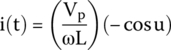
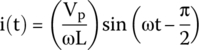
By applying this concept on the main equation, we get the final equation for the current across the inductor.
10.12 Out of Sync
In this chapter, we have learned that the forces generated by inductors every time current changes for less or for more create a kind of inertia. This inertia creates a delay between current and voltage variations across the inductor. When voltage is maximum, current is minimum and vice versa. Current variations are always delayed compared to voltage in an inductor.
Observing equations (10.2) and (10.3), we see that the first equation describes voltages in terms of sin(ωt) and that the second one describes current in terms of ![]() .
.
The existence of ![]() , in the current equation, equivalent to −90°, tells us that the current is 90° delayed compared to voltage.
, in the current equation, equivalent to −90°, tells us that the current is 90° delayed compared to voltage.
Figure 10.12 shows a graph of current (second curve) delayed 90° in relation to voltage (first curve).
Figure 10.12 Current behind voltage in an inductor.
Exercises
- What is the equivalent inductance of three inductors in series with 100 mH, 1 μH, and 12 mH?
- What is the equivalent inductance of three inductors in parallel with 100 mH, 1 μH, and 12 mH?
- A 40 Hz alternating voltage is applied to a 12 mH inductor. Find the inductive reactance for this frequency.
- A 12 V peak and 50 Hz alternating voltage is applied to a 12 mH inductor. Find the current across the inductor for t = 2s.
Solutions
- Series inductance can be calculated by the following formula:
Hence,

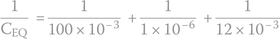
- Parallel inductance can be calculated by the following formula:

Hence,
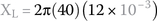
- Inductive reactance can be found by the following formula:

Upon substituting the values, we get
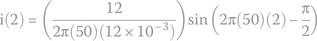
- We can find the current using the respective current equation:
or

Notes
- 1 In honor of Joseph Henry (1797–1878), American scientist who discovered electromagnetic induction, independently, at the same time as Michael Faraday (1791–1867) in England.
- 2 In honor of his pioneering work in electromagnetism.
- 3 An ideal inductor has zero electric resistance.
- 4 Hypothetical situation for an ideal inductor with zero resistance. In real life, voltage will stabilize in a very small value.
- 5 For the ideal resistor, obviously. In real life, the inductor will be seen as a very small resistor.
..................Content has been hidden....................
You can't read the all page of ebook, please click here login for view all page.