Unfortunately, the naming of these two libraries is rather confusing. GDAL, which stands for Geospatial Data Abstraction Library, was originally just a library for working with raster geo-spatial data, while the separate OGR library was intended to work with vector data. However, the two libraries are now partially merged, and are generally downloaded and installed together under the combined name of GDAL. To avoid confusion, we will call this combined library GDAL/OGR and use GDAL to refer to just the raster translation library.

A default installation of GDAL supports reading 81 different raster file formats and writing to 41 different formats. OGR by default supports reading 27 different vector file formats and writing to 15 formats. This makes GDAL/OGR one of the most powerful geo-spatial data translators available, and certainly the most useful freely-available library for reading and writing geo-spatial data.

GDAL design

GDAL uses the following data model for describing raster geo-spatial data:

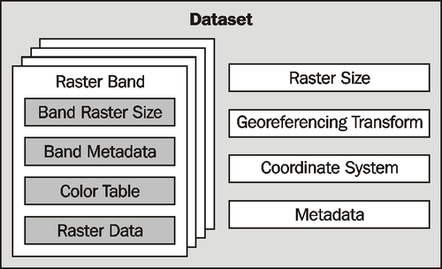
Let's take a look at the various parts of this model:

1. A dataset holds all the raster data, in the form of a collection of raster "bands", and information that is common to all these bands. A dataset normally represents the contents of a single file.
2. A raster band represents a band, channel, or layer within the image. For example, RGB image data would normally have separate bands for the red, green, and blue components of the image.
3. The raster size specifies the overall width of the image in pixels and the overall height of the image in lines.
4. The georeferencing transform converts from (x,y) raster coordinates into georeferenced coordinates—that is, coordinates on the surface of the Earth. There are two types of georeferencing transforms supported by GDAL: affine transformations and ground control points.

   An affine transformation is a mathematical formula allowing the following operations to be applied to the raster data:

   

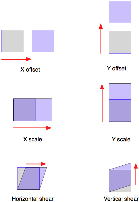
   More than one of these operations can be applied at once; this allows you to perform sophisticated transforms such as rotations.

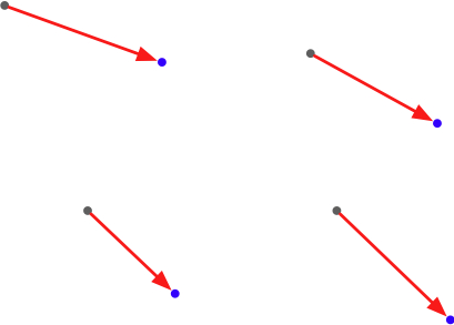
   Ground Control Points (GCPs) relate one or more positions within the raster to their equivalent georeferenced coordinates, as shown in the following figure:

   
   • Note that GDAL does not translate coordinates using GCPs—that is left up to the application, and generally involves complex mathematical functions to perform the transformation.
5. The coordinate system describes the georeferenced coordinates produced by the georeferencing transform. The coordinate system includes the projection and datum as well as the units and scale used by the raster data.
6. The metadata contains additional information about the dataset as a whole.

Each raster band contains (among other things):

1. The band raster size. This is the size (number of pixels across and number of lines high) for the data within the band. This may be the same as the raster size for the overall dataset, in which case the dataset is at full resolution, or the band's data may need to be scaled to match the dataset.
2. Some band metadata providing extra information specific to this band.
3. A color table describing how pixel values are translated into colors.
4. The raster data itself.

GDAL provides a number of drivers that allow you to read (and sometimes write) various types of raster geo-spatial data. When reading a file, GDAL selects a suitable driver automatically based on the type of data; when writing, you first select the driver and then tell the driver to create the new dataset you want to write to.

from osgeo import gdal,gdalconst
import struct

dataset = gdal.Open("DEM.dat")
band = dataset.GetRasterBand(1)

fmt = "<" + ("h" * band.XSize)

totHeight = 0

for y in range(band.YSize):
    scanline = band.ReadRaster(0, y, band.XSize, 1,
                               band.XSize, 1,
                               band.DataType)
    values = struct.unpack(fmt, scanline)

    for value in values:
        totHeight = totHeight + value

average = totHeight / (band.XSize * band.YSize)
print "Average height =", average

OGR design

OGR uses the following model for working with vector-based geo-spatial data:

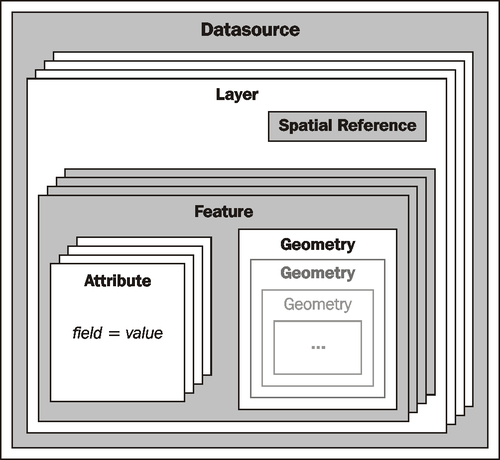
Let's take a look at this design in more detail:

1. The datasource represents the file you are working with—though it doesn't have to be a file. It could just as easily be a URL or some other source of data.
2. The datasource has one or more layers, representing sets of related data. For example, a single datasource representing a country may contain a terrain layer, a contour lines layer, a roads layer, and a city boundaries layer. Other datasources may consist of just one layer. Each layer has a spatial reference and a list of features.
3. The spatial reference specifies the projection and datum used by the layer's data.
4. A feature corresponds to some significant element within the layer. For example, a feature might represent a state, a city, a road, an island, and so on. Each feature has a list of attributes and a geometry.
5. The attributes provide additional meta-information about the feature. For example, an attribute might provide the name for a city feature, its population, or the feature's unique ID used to retrieve additional information about the feature from an external database.
6. Finally, the geometry describes the physical shape or location of the feature. Geometries are recursive data structures that can themselves contain sub-geometries—for example, a country feature might consist of a geometry that encompasses several islands, each represented by a sub-geometry within the main "country" geometry.

   The Geometry design within OGR is based on the Open Geospatial Consortium's Simple Features model for representing geo-spatial geometries. For more information, see http://www.opengeospatial.org/standards/sfa.

Like GDAL, OGR also provides a number of drivers that allow you to read (and sometimes write) various types of vector-based geo-spatial data. When reading a file, OGR selects a suitable driver automatically; when writing, you first select the driver and then tell the driver to create the new datasource to write to.

from osgeo import ogr

shapefile = ogr.Open("TM_WORLD_BORDERS-0.3.shp")
layer = shapefile.GetLayer(0)

for i in range(layer.GetFeatureCount()):
    feature = layer.GetFeature(i)
    name = feature.GetField("NAME")
    geometry = feature.GetGeometryRef()
    print i, name, geometry.GetGeometryName()

GDAL and OGR are well-documented, but with a catch for Python programmers. The GDAL/OGR library and associated command-line tools are all written in C and C++. Bindings are available that allow access from a variety of other languages, including Python, but the documentation is all written for the C++ version of the libraries. This can make reading the documentation rather challenging—not only are all the method signatures written in C++, but the Python bindings have changed many of the method and class names to make them more "pythonic".

Fortunately, the Python libraries are largely self-documenting, thanks to all the docstrings embedded in the Python bindings themselves. This means you can explore the documentation using tools such as Python's built-in pydoc utility, which can be run from the command line like this:

pydoc -g osgeo

This will open up a GUI window allowing you to read the documentation using a web browser. Alternatively, if you want to find out about a single method or class, you can use Python's built-in help() command from the Python command line, like this:

>>> import osgeo.ogr
>>> help(osgeo.ogr.Datasource.CopyLayer)

Not all the methods are documented, so you may need to refer to the C++ docs on the GDAL website for more information. Some of the docstrings present are copied directly from the C++ documentation—but, in general, the documentation for GDAL/OGR is excellent, and should allow you to quickly come up to speed using this library.

GDAL/OGR runs on modern Unix machines, including Linux and Mac OS X as well as most versions of Microsoft Windows. The main website for GDAL can be found at:

http://gdal.org

And the main website for OGR is http://gdal.org/ogr

To download GDAL/OGR, follow the Downloads link on the main GDAL website. Windows users may find the "FWTools" package useful as it provides a wide range of geo-spatial software for win32 machines, including GDAL/OGR and its Python bindings. FWTools can be found at:

http://fwtools.maptools.org

For those running Mac OS X, pre-built binaries for GDAL/OGR can be obtained from:

http://www.kyngchaos.com/software/frameworks

Make sure that you install GDAL version 1.7 or later as you will need this version to work through the examples in this book.

Being an open source package, the complete source code for GDAL/OGR is available from the website, so you can compile it yourself. Most people, however, will simply want to use a pre-built binary version.