Imagine that you have a database containing a range of geo-spatial data for San Francisco. This database might include geographical features, roads and the location of prominent buildings and other man-made features such as bridges, airports, and so on.

Such a database can be a valuable resource for answering various questions. For example:

Many of these types of problems can be solved using tools such as the PostGIS spatially-enabled database. For example, to calculate the total area of the Golden Gate Park, you might use the following SQL query:

select ST_Area(geometry) from features
  where name = “Golden Gate Park”;

To calculate the distance between two places, you first have to geocode the locations to obtain their latitude and longitude. There are various ways to do this; one simple approach is to use a free geocoding web service such as this:

http://tinygeocoder.com/create-api.php?q=Pier 39,San Francisco,CA

This returns a latitude value of 37.809662 and a longitude value of -122.410408.

Similarly, we can find the location of the Moscone Center using this query:

http://tinygeocoder.com/create-api.php?q=Moscone Center, San Francisco, CA

This returns a latitude value of 37.784161 and a longitude value of -122.401489.

Now that we have the coordinates for the two desired locations, we can calculate the distance between them using the pyproj Python library:

import pyproj

lat1,long1 = (37.809662,-122.410408)
lat2,long2 = (37.784161,-122.401489)

geod = pyproj.Geod(ellps="WGS84")
angle1,angle2,distance = geod.inv(long1, lat1, long2, lat2)

print "Distance is %0.2f meters" % distance

This prints the distance between the two points:

Distance is 2937.41 meters

Of course, you wouldn't normally do this sort of analysis on a one-off basis like this—it's much more common to create a Python program that will answer these sorts of questions for any desired set of data. You might, for example, create a web application that displays a menu of available calculations. One of the options in this menu might be to calculate the distance between two points; when this option is selected, the web application would prompt the user to enter the two locations, attempt to geocode them by calling an appropriate web service (and display an error message if a location couldn't be geocoded), then calculate the distance between the two points using Proj, and finally display the results to the user.

Alternatively, if you have a database containing useful geo-spatial data, you could let the user select the two locations from the database rather than typing in arbitrary location names or street addresses.

However you choose to structure it, performing calculations like this will usually be a major part of your geo-spatial application.

Imagine that you wanted to see which areas of a city are typically covered by a taxi during an average working day. You might place a GPS recorder into a taxi and leave it to record the taxi's position over several days. The results would be a series of timestamp, latitude and longitude values like the following:

2010-03-21 9:15:23  -38.16614499  176.2336626
2010-03-21 9:15:27  -38.16608632  176.2335635
2010-03-21 9:15:34  -38.16604198  176.2334771
2010-03-21 9:15:39  -38.16601507  176.2333958
...

By themselves, these raw numbers tell you almost nothing. But, when you display this data visually, the numbers start to make sense:

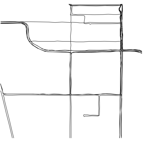
You can immediately see that the taxi tends to go along the same streets again and again. And, if you draw this data as an overlay on top of a street map, you can see exactly where the taxi has been:

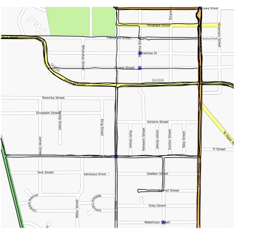
(Street map courtesy of http://openstreetmap.org).

While this is a very simple example, visualization is a crucial aspect of working with geo-spatial data. How data is displayed visually, how different data sets are overlaid, and how the user can manipulate data directly in a visual format are all going to be major topics of this book.

The concept of a "mash-up" has become popular in recent years. Mash-ups are applications that combine data and functionality from more than one source. For example, a typical mash-up may combine details of houses for rent in a given city, and plot the location of each rental on a map, like this:

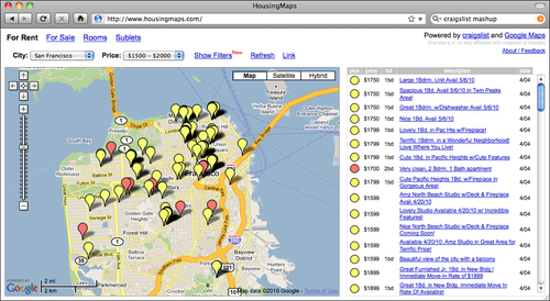
This example comes from http://housingmaps.com.

The Google Maps API has been immensely popular in creating these types of mash-ups. However, Google Maps has some serious licensing and other limitations. It is not the only option—tools such as Mapnik, open layers, and MapServer, to name a few, also allow you to create mash-ups that overlay your own data onto a map.

Most of these mash-ups run as web applications across the Internet, running on a server that can be accessed by anyone who has a web browser. Sometimes, the mash-ups are private, requiring password access, but usually they are publically available and can be used by anyone. Indeed, many businesses (such as the rental mashup shown above) are based on freely-available geo-spatial mash-ups.