
In this section, we will examine the Python interface to the Mapnik toolkit in much more detail. The Python documentation for Mapnik (http://media.mapnik.org/api_docs/python) is confusing and incomplete, so you may find this section to be a useful reference guide while writing your own Mapnik-based programs.
Note
The Mapnik toolkit is written in C++ and provides bindings to let you access it via Python. Not every feature implemented in Mapnik is available from Python; only those features that are available and relevant to the Python developer will be discussed here.
Before you can access a given set of geo-spatial data within a map, you need to set up a Mapnik Datasource object. This acts as a "bridge" between Mapnik and your geo-spatial data:
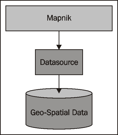
You typically create the datasource using one of the convenience constructors described below. Then you add that datasource to any Mapnik layer objects which will use that data:
layer.datasource = datasource
A single datasource object can be shared by multiple layers, or it can be used by just one layer.
There are many different types of datasources supported by Mapnik, some of which are experimental or access data in commercial databases. Let's take a closer look at the types of datasources you are likely to find useful.
It is easy to use a Shapefile as a Mapnik datasource. All you need to do is supply the name and directory path for the desired Shapefile to the mapnik.Shapefile() convenience constructor:
import mapnik
...
datasource = mapnik.Shapefile(file="shapefile.shp")
If the Shapefile is in a different directory, you can use os.path.join() to define the full path. For example, you can open a Shapefile in a directory relative to your Python program like this:
datasource = mapnik.Shapefile(file=os.path.join("..", "data",
                                                "shapes.shp"))
When you open a Shapefile datasource, the Shapefile's attributes can be used within a filter expression, and as fields to be displayed by a TextSymbolizer. By default, all text within the Shapefile will be assumed to be in UTF-8 character encoding; if you need to use a different character encoding, you can use the encoding parameter, like this:
datasource = mapnik.Shapefile(file="shapefile.shp",
                              encoding="latin1")
This datasource allows you to use data from a PostGIS database on your map. The basic usage of the PostGIS datasource is like this:
import mapnik
...
datasource = mapnik.PostGIS(user="..." password="...",
                            dbname="...", table="...")
You simply supply the username and password used to access the PostGIS database, the name of the database, and the name of the table that contains the spatial data you want to include on your map. As with the Shapefiles, the fields in the database table can be used inside a filter expression, and as fields to be displayed using a TextSymbolizer.
There are some performance issues to be aware of when retrieving data from a PostGIS database. Imagine that we're accessing a large database table, and use the following to generate our map's layer:
datasource = mapnik.PostGIS(user="...", password="...",
                            dbname="...", table="myBigTable")

layer = mapnik.Layer("myLayer")
layer.datasource = datasource
layer.styles.append("myLayerStyle")

symbol = mapnik.PolygonSymbolizer(mapnik.Color("#406080"))

rule = mapnik.Rule()
rule.filter = mapnik.Filter("[level] = 1")
rule.symbols.append(symbol)

style = mapnik.Style()
style.rules.append(rule)

map.append_style("myLayerStyle", style)
Notice how the datasource refers to the myBigTable table within the PostGIS database, and we use a filter expression ([level] = 1) to select the particular records within that database table to be displayed using our PolygonSymbolizer.
When rendering this map layer, Mapnik will scan through every record in the table, apply the filter expression to each record in turn, and then use the PolygonSymbolizer to draw the record's polygon if, and only if, the record matches the filter expression. This is fine if there aren't many records in the table, or if most of the records will match the filter expression. But, imagine that the myBigTable table contains a million records, with only 10,000 records having a level value of 1. In this case, Mapnik will scan through the entire table and discard ninety-nine percent of the records. Only the remaining one percent will actually be drawn.
As you can imagine, this is extremely inefficient. Mapnik will waste a lot of time filtering the records in the database when PostGIS itself is much better suited to the task. In situations like this, you can make use of a sub-select query so that the database itself will do the filtering before the data is received by Mapnik. We actually used a sub-select query in the previous chapter, where we retrieved tiled shoreline data from our PostGIS database, though we didn't explain how it worked in any depth.
To use a sub-select query, you replace the table name with an SQL select statement that does the filtering and returns the fields needed by Mapnik to generate the map's layer. Here is an updated version of the last example, which uses a sub-select query:
query = "(select geom from myBigTable where level=1) as data"
datasource = mapnik.PostGIS(user="...", password="...",
                            dbname="...", table=query)

layer = mapnik.Layer("myLayer")
layer.datasource = datasource
layer.styles.append("myLayerStyle")

symbol = mapnik.PolygonSymbolizer(mapnik.Color("#406080"))

rule = mapnik.Rule()
rule.symbols.append(symbol)

style = mapnik.Style()
style.rules.append(rule)

map.append_style("myLayerStyle", style)
We've replaced the table name with a PostGIS sub-select statement that filters out all records with a level value not equal to 1 and returns just the geom field for the matching records back to Mapnik. We've also removed the rule.filter = line in our code as the datasource will only ever return records that already match that filter expression.
Note
Note that the sub-select statement ends with ...as data. We have to give the results of the sub-select statement a name, even though that name is ignored. In this case, we've called the results data, though you can use any name you like.
If you use a sub-select, it is important that you include all the fields used by your filter expressions and symbolizers. If you don't include a field in the sub-select statement, it won't be available for Mapnik to use.
The GDAL datasource allows you to include any GDAL-compatible raster image datafile within your map. The GDAL datasource is straightforward to use:
datasource = mapnik.Gdal(file="myRasterImage.tiff")
Once you have a GDAL datasource, you need to use a RasterSymbolizer to draw it onto the map:
layer = mapnik.Layer("myLayer")
layer.datasource = datasource
layer.styles.append("myLayerStyle")

symbol = mapnik.RasterSymbolizer()

rule = mapnik.Rule()
rule.symbols.append(symbol)

style = mapnik.Style()
style.rules.append(rule)

map.append_style("myLayerStyle", style)
The OGR datasource lets you display any OGR-compatible vector data on your map. The convenience constructor for an OGR datasource requires at least two named parameters:
datasource = mapnik.Ogr(file="...", layer="...")
The file parameter is the name of an OGR-compatible datafile, while layer is the name of the desired layer within that datafile. You could use this, for example, to read a Shapefile via the OGR driver:
datasource = mapnik.Ogr(file="shapefile.shp",
                        layer="shapefile")
More usefully, you can use this to load data from any vector-format datafile supported by OGR. The various supported formats are listed on the following web page:
Of particular interest to us is the Virtual Datasource (VRT) format. The VRT format is an XML-formatted file which allows you to set up an OGR datasource that isn't stored in a simple file on disk. We saw in the previous chapter how this can be used to display data from a MySQL database on a map, despite the fact that Mapnik itself does not implement a MySQL datasource.
The VRT file format is relatively complex, though it is explained fully on the OGR website. Here is an example of how you can use a VRT file to set up a MySQL virtual datasource:
<OGRVRTDataSource>
  <OGRVRTLayer name="myLayer">
    <SrcDataSource>MYSQL:mydb,user=user,password=pass,
                   tables=myTable</SrcDataSource>
    <SrcSQL>
      SELECT name,geom FROM myTable
    </SrcSQL>
  </OGRVRTLayer>
</OGRVRTDataSource>
The<SrcDataSource> element contains a string that sets up the OGR MySQL datasource. This string is of the format:
MySQL:«dbName»,user=«username»,password=«pass»,tables=«tables»
You need to replace"dbName" with the name of your database,"username" and"pass" with the username and password used to access your MySQL database, and"tables" with a list of the database tables you want to retrieve your data from. If you are retrieving data from multiple tables, you need to separate the table names with a semicolon, such as:
tables=lakes;rivers;coastlines
Note that all the text between<SrcDataSource> and</SrcDataSource> must be on a single line.
The text inside the<SrcSQL> element should be a MySQL select statement that retrieves the desired information from the database table(s). As with the PostGIS datasource, you can use this to filter out unwanted records before they are passed to Mapnik, which will significantly improve performance.
The VRT file should be saved to disk. For example, the above virtual file definition might be saved to a file named myLayer.vrt. You would then use this file to define your OGR datasource, such as:
datasource = mapnik.Ogr(file="myLayer.vrt", layer="myLayer")
The SQLite datasource allows you to include data from an SQLite (or SpatiaLite) database on a map. The mapnik.SQLite() convenience constructor accepts a number of keyword parameters; the ones most likely to be useful are:
file="...":The name and optional path to the SQLite database filetable="...":The name of the desired table within this databasegeometry_field="...":The name of a field within this table that holds the geometry to be displayedkey_field="...":The name of the primary key field within the table
For example, to access a table named countries in a SpatiaLite database named mapData.db, you might use the following:
datasource = mapnik.SQLite(file="mapData.db",
                           table="countries",
                           geometry_field="outline",
                           key_field="id")
All of the fields within the countries table will be available for use in Mapnik filters and for display using a TextSymbolizer. The various symbolizers will use the geometry stored in the outline field for drawing lines, polygons, and so on.
The OSM datasource allows you to include OpenStreetMap data onto a map. The OpenStreetMap data is stored in .OSM format, which is an XML format containing the underlying nodes, ways, and relations used by OpenStreetMap. The OpenStreetMap data format, and options for downloading .OSM files, can be found at:
If you have downloaded a .OSM file and want to access it locally, you can set up your datasource by using:
datasource = mapnik.OSM(file="myData.osm")
If you wish to use an OpenStreetMap API call to retrieve the OSM data on the fly, you can do this by supplying a URL to read the data from, along with a bounding box to identify which set of data you want to download. For example:
osmURL = "http://api.openstreetmap.org/api/0.6/map"
bounds = "176.193,-38.172,176.276,-38.108"
datasource = mapnik.OSM(url=osmURL, bbox=bounds)
The bounding box is a string containing the left, bottom, right, and top coordinates for the desired bounding box, respectively.
The PointDatasource is a relatively recent addition to Mapnik. It allows you to manually define a set of data points that will appear on your map.
Setting up a point datasource is easy; you simply create the PointDatasource object:
datasource = mapnik.PointDatasource()
You then use the PointDatasource's add_point() method to add the individual points to the datasource. This method takes four parameters:
long:The point's longitudelat:The point's latitudekey:The name of the attribute for this pointvalue:The value of the attribute for this point
You would normally use the same key for each data point, and set the value to some appropriate string that you can then display on your map. For example, the following code combines a PointDatasource with a TextSymbolizer to place labels onto a map at specific lat/long coordinates:
datasource = mapnik.PointDatasource()

datasource.add_point(-0.126, 51.513, "label", "London")
datasource.add_point(-2.591, 51.461, "label", "Bristol")
datasource.add_point(1.2964, 52.630, "label", "Norwich")
...

layer = mapnik.Layer("points")
layer.datasource = datasource
layer.styles.append("pointStyle")

symbol = mapnik.TextSymbolizer("label", "DejaVu Sans Bold",
                               10, mapnik.Color("#000000"))

rule = mapnik.Rule()
rule.symbols.append(symbol)

style = mapnik.Style()
style.rules.append(rule)

map.append_style("pointStyle", style)
As we saw earlier in this chapter, Mapnik uses rules to specify which particular symbolizers will be used to render a given feature. Rules are grouped together into a style, and the various styles are added to your map and then referred to by name when you set up your Layer. In this section, we will examine the relationship between rules, filters, and styles, and see just what can be done with these various Mapnik classes.
Let's take a closer look at Mapnik's Rule class. A Mapnik rule has two parts: a set of conditions, and a list of symbolizers. If the rule's conditions are met then the symbolizers will be used to draw the matching features onto the map.
There are three types of conditions supported by a rule:
- A Mapnik filter can be used to specify an expression that must be met by the feature if it is to be drawn.
- The rule itself can specify minimum and maximum scale denominators that must apply. This can be used to set up rules that are only used if the map is drawn at a given scale.
- The rule can have an else condition, which means that the rule will only be applied if no other rule in the style has had its conditions met.
If all the conditions for a rule are met then the associated list of symbolizers will be used to render the feature onto the map.
Let's take a look at these conditions in more detail.
Mapnik's Filter() constructor takes a single parameter: a string defining an expression that the feature must match if the rule is to apply. You then store the returned filter object into the rule's filter attribute:
rule.filter = mapnik.Filter("...")
Let's consider a very simple filter expression, comparing a field or attribute against a specific value:
filter = mapnik.Filter("[level] = 1")
String values can be compared by putting single quote marks around the value, such as:
filter = mapnik.Filter("[type] = 'CITY'")
Note that the field name and value are both case-sensitive, and that you must surround the field or attribute name with square brackets.
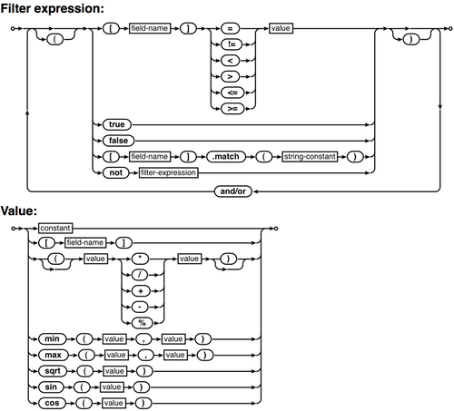
Of course, simply comparing a field with a value is the most basic type of comparison you can do. Filter expressions have their own powerful and flexible syntax for defining conditions, similar in concept to an SQL where expression. The following syntax diagram describes all the options for writing filter expression strings:
Consider the following two maps:
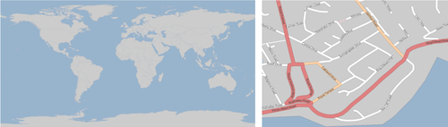
Obviously, there's no point in drawing streets onto a map of the entire world. Similarly, the country outlines shown on the world map are at too large a scale to draw detailed coastlines for an individual city. But, if your application allows the user to zoom in from the world map right down to an individual street, you will need to use a single set of Mapnik styles to generate the map regardless of the scale at which you are drawing it.
Mapnik allows you to do this by selectively displaying features based on the map's scale denominator. If you had a map printed on paper at 1:100,000 scale, then the scale denominator would be the number after the colon (100,000 in this case). Drawing maps digitally makes this a bit more complicated, but the idea remains the same.
A Mapnik rule can have a minimum and maximum scale denominator value associated with it:
rule.min_scale = 10000
rule.max_scale = 100000
If the minimum and maximum scale denominators are set then the rule will only apply if the map's scale denominator is within this range.
You can also apply minimum and maximum scale factors to an entire layer:
layer.minzoom = 1.0/100000
layer.maxzoom = 1.0/200000
Tip
Note that rules use scale denominators while layers use scale factors. This can be rather confusing as the relationship between the two is not straightforward. For more information on scale factors and scale denominators, please refer to http://trac.mapnik.org/wiki/ScaleAndPpi.
The whole layer will only be displayed when the map's current scale factor is within this range. This is useful if you have a datasource that should only be used when displaying the map at a certain scale—for example, only using high-resolution shoreline data when the user has zoomed in.
Scale denominators can be used intuitively. For example, a scale denominator value of 200,000 represents a map drawn at roughly 1:200,000 scale. But, this is only an approximation; the actual calculation of a scale denominator has to take into account two important factors:
- Because Mapnik renders a map as a bitmapped image, the size of the individual pixels within the image comes into play. Since bitmapped images can be displayed on a variety of different computer screens with different pixel sizes, Mapnik uses a standardized rendering pixel size as defined by the Open Geospatial Consortium to define how big a pixel is going to be. This value is 0.28 mm, and is approximately the size of a pixel on modern video displays.
- The map projection being used can have a huge effect on the calculated scale denominator. Map projections always distort true distances, and a projection that is accurate at the equator may be wildly inaccurate closer to the Poles.
Depending on the projection being used, the formula Mapnik uses to calculate the scale denominator can get rather complicated. Rather than worrying about the formulas, it is much easier just to ask Mapnik to calculate the scale denominator and scale factor for us:
map = mapnik.Map(width, height, projection)
map.zoom_to_box(bounds)
print map.scale_denominator(), map.scale()
You can then zoom the map to your desired scale and see what the scale factor and denominator are, which you can then plug into your styles to choose which features should be displayed at a given scale denominator range.
Imagine that you want to draw some features in one color, and all other features in a different color. One way to achieve this is to use Mapnik rules, as shown here:
rule1.filter = mapnik.Filter("[level] = 1")
...
rule2.filter = mapnik.Filter("[level] != 1")
This is fine for simple filter expressions, but when the expressions get more complicated it is a lot easier to use an "else" rule, as shown in the following snippet:
rule1.filter = mapnik.Filter("[level] = 1")
...
rule2.set_else(True)
If you call set_else(True) for a rule, that rule be used if, and only if, no previous rule in the same style has had its filter conditions met.
Else rules are particularly useful if you have a number of filter conditions and want to have a "catch-all" rule at the end that will apply if no other rule has been used to draw the feature. For example:
rule1.filter = mapnik.Filter("[type] = 'city'")
rule2.filter = mapnik.Filter("[type] = 'town'")
rule3.filter = mapnik.Filter("[type] = 'village'")
rule4.filter.set_else(True)
Symbolizers are used to draw features onto a map. In this section, we will look at how you can use the various types of symbolizers to draw lines, polygons, labels, points, and images.
There are two Mapnik symbolizers that can be used to draw lines onto a map: LineSymbolizer and LinePatternSymbolizer. Let's look at each of these in turn.
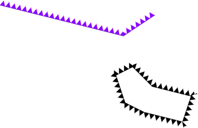
The LineSymbolizer draws linear features and traces around the outline of polygons, as shown in the following image:
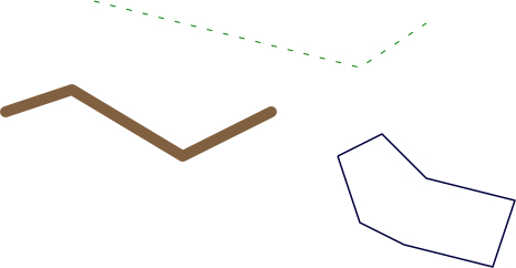
The LineSymbolizer is one of the most useful of the Mapnik symbolizers. Here is the Python code that created the LineSymbolizer used to draw the dashed line in the last example:
stroke = mapnik.Stroke()
stroke.color = mapnik.Color("#008000")
stroke.width = 1.0
stroke.add_dash(5, 10)
symbolizer = mapnik.LineSymbolizer(stroke)
As you can see, the LineSymbolizer uses a Mapnik Stroke object to define how the line will be drawn. To use a LineSymbolizer, you first create the stroke object and set the various options for how you want the line to be drawn. You then create your LineSymbolizer, passing the stroke object to the LineSymbolizer's constructor:
symbolizer = mapnik.LineSymbolizer(stroke)
Let's take a closer look at the various line-drawing options provided by the stroke object.
By default, lines are drawn in black. You can change this by setting the stroke's color attribute to a Mapnik color object:
stroke.color = mapnik.Color("red")
For more information about the Mapnik color object, and the various ways in which you can specify a color, please refer to the Using Colors section later in this chapter.
The line drawn by a LineSymbolizer will be one pixel wide by default. To change this, set the stroke's width attribute to the desired width, in pixels:
stroke.width = 1.5
Note that you can use fractional line widths for fine-grained control of your line widths.
You can change how opaque or transparent the line is by setting the stroke's opacity attribute:
stroke.opacity = 0.8
The opacity can range from 0.0 (completely transparent) to 1.0 (completely opaque). If the opacity is not specified, the line will be completely opaque.
The line cap specifies how the ends of the line should be drawn. Mapnik supports three standard line cap settings:
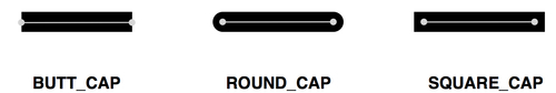
By default, the lines will use BUTT_CAP style, but you can change this by setting the stroke's line_cap attribute, such as:
stroke1.line_cap = mapnik.line_cap.BUTT_CAP
stroke2.line_cap = mapnik.line_cap.ROUND_CAP
stroke3.line_cap = mapnik.line_cap.SQUARE_CAP
When a line changes direction, the "corner" of the line can be drawn in one of three standard ways:
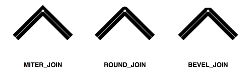
The default behavior is to use MITER_JOIN, but you can change this by setting the stroke's line_join attribute to a different value:
stroke1.line_join = mapnik.line_join.MITER_JOIN
stroke2.line_join = mapnik.line_join.ROUND_JOIN
stroke3.line_join = mapnik.line_join.BEVEL_JOIN
You can add "breaks" to a line to make it appear dashed or dotted. To do this, you add one or more dash segments to the stroke. Each dash segment defines a dash length and a gap length; the line will be drawn for the given dash length, and will then leave a gap of the specified length before continuing to draw the line:
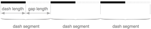
You add a dash segment to a line by calling the stroke's add_dash() method:
stroke.add_dash(5, 5)
This will give the line a five-pixel dash followed by a five-pixel gap.
You aren't limited to just having a single dash segment; if you call add_dash() multiple times, you will create a line with more than one segment. These dash segments will be processed in turn, allowing you to create varying patterns of dashes and dots. For example:
stroke.add_dash(10, 2)
stroke.add_dash(2, 2)
stroke.add_dash(2, 2)
would result in the following repeating line pattern:
Note
Drawing roads and other complex linear features
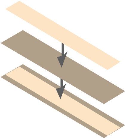
One thing that may not be immediately obvious is that you can draw a road onto a map by overlying two LineSymbolizers; the first LineSymbolizer draws the edges of the road, while the second LineSymbolizer draws the road's interior. For example:
stroke = mapnik.Stroke()
stroke.color = mapnik.Color("#bf7a3a")
stroke.width = 7.0
roadEdgeSymbolizer = mapnik.LineSymbolizer(stroke)

stroke = mapnik.Stroke()
stroke.color = mapnik.Color("#ffd3a9")
stroke.width = 6.0
roadInteriorSymbolizer = mapnik.LineSymbolizer(stroke)
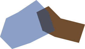
This technique is commonly used for drawing street maps. The two symbolizers that we just defined would then be overlaid to produce a road, as shown in the following image:
Note
This technique can be used for more than just drawing roads; the creative use of symbolizers is one of the main "tricks" to achieving complex visual effects using Mapnik.
The LinePatternSymbolizer is used in those special situations where you want to draw a line that can't be rendered using a simple Stroke object. The LinePatternSymbolizer accepts a PDF or TIFF format image file, and draws that image repeatedly along the length of the line or around the outline of a polygon:
Notice that linear features and polygon boundaries have a direction—that is, the line or polygon border moves from one point to the next in the order in which the points were defined when the geometry was created. For example, the points that make up the line segment at the top of the above illustration were defined from left to right—that is, the leftmost point is defined first, then the middle point, and then the rightmost point.
The direction of a feature is important as it affects the way the LinePatternSymbolizer draws the image. If the linestring that we just saw was defined in the opposite direction, the LinePatternSymbolizer would draw it like this:

As you can see, the LinePatternSymbolizer draws the image oriented towards the left of the line as it moves from one point to the next. To draw the image oriented towards the right, you will have to reverse the order of the points within your feature.
To use a LinePatternSymbolizer within your Python code, you simply create an instance of mapnik.LinePatternSymbolizer and give it the name of the image file, the file format (PNG or TIFF), and the pixel dimensions of the image:
symbolizer = mapnik.LinePatternSymbolizer("image.png",
                                          "png", 11, 11)
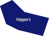
Just as there are two symbolizers to draw lines, there are two symbolizers to draw the interior of a polygon: the PolygonSymbolizer and the PolygonPatternSymbolizer. Let's take a closer look at each of these two symbolizers.
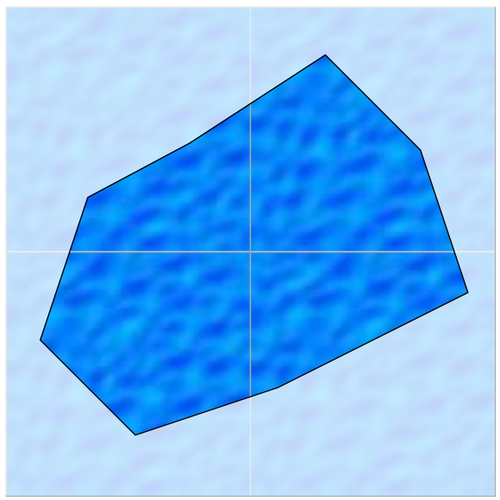
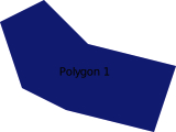
A PolygonSymbolizer fills the interior of a polygon with a single color:
You create a PolygonSymbolizer in the following way:
symbolizer = mapnik.PolygonSymbolizer()
Let's take a closer look at the various options for controlling how the polygon will be drawn.
By default, a PolygonSymbolizer will draw the interior of the polygon in grey. To change the color used to fill the polygon, set the PolygonSymbolizer's fill attribute to the desired Mapnik color object:
symbolizer.fill = mapnik.Color("red")
For more information about creating Mapnik color objects, please refer to the Using colors section later in this chapter.
By default, the polygon will be completely opaque. You can change this by setting the PolygonSymbolizer's opacity attribute:
symbolizer.fill_opacity = 0.5
The opacity can range from 0.0 (completely transparent) to 1.0 (completely opaque). In the previous illustration, the left polygon had an opacity of 0.5.
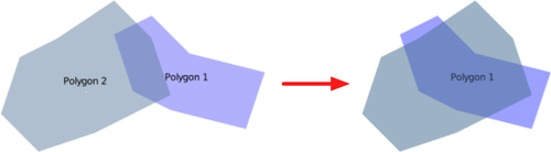
Gamma correction is an obscure concept, but can be very useful at times. If you draw two polygons that touch with exactly the same fill color, you will still see a line between the two, as shown in the following image:
This is because of the way Mapnik anti-aliases the edges of the polygons. If you want these lines between adjacent polygons to disappear, you can add a gamma correction factor:
symbolizer.gamma = 0.63
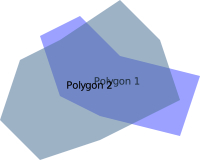
This results in the two polygons appearing as one:

It may take some experimenting, but using a gamma value of around 0.5 to 0.7 will generally remove the ghost lines between adjacent polygons. The default value of 1.0 means that no gamma correction will be performed at all.
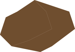
The PolygonPatternSymbolizer fills the interior of a polygon using a supplied image file:
The image will be tiled—that is, drawn repeatedly to fill in the entire interior of the polygon:
Because the right side of one tile will appear next to the left side of the adjacent tile, and the bottom of the tile will appear immediately above the top of the tile below it (and vice versa), you need to choose an appropriate image that will look good when it is drawn in this way.
Using the PolygonPatternSymbolizer is easy; as with the LinePatternSymbolizer, you create a new instance and give it the name of your image file, the file format (PNG or TIFF), and the width and height of the image:
symbolizer = mapnik.PolygonPatternSymbolizer("image.png",
                                             "png", 102, 80)
Textual labels are an important part of any map. In this section, we will explore the TextSymbolizer, which draws text onto a map.
Note
The ShieldSymbolizer also allows you to draw labels, combining text with an image. We will look at the ShieldSymbolizer in the section on drawing points, below.
The TextSymbolizer allows you to draw text onto point, line, and polygon features:

The basic usage of a TextSymbolizer is quite simple. For example, the polygon in the last illustration was labeled using the following code:
symbolizer = mapnik.TextSymbolizer("label",
                                   "DejaVu Sans Book", 10,
                                   mapnik.Color("black"))
This symbolizer will display the value of the feature's label field using the given font, font size, and color. Whenever you create a TextSymbolizer object, you must provide these four parameters.
Let's take a closer look at these parameters, as well as the other options you have for controlling how the text will be displayed.
You select the text to be displayed by passing a field or attribute name as the first parameter to the TextSymbolizer's constructor. Note that the text will always be taken from the underlying data; there is no option for hardwiring a label into your rule.
The label will be drawn using a font and font size you specify when you create the TextSymbolizer object. You have two options for selecting a font: you can use one of the built-in fonts supplied by Mapnik, or you can install your own custom font.
To find out what fonts are available, run the following program:
import mapnik
for font in mapnik.FontEngine.face_names():
    print font
You can find out more about the process involved in installing a custom font on the following web page:
Note that the font is specified by name, and that the font size is in points.
You can control how opaque or transparent the text is by setting the opacity attribute, as shown here:
symbolizer.opacity = 0.5
The opacity ranges from 0.0 (completely transparent) to 1.0 (completely opaque).
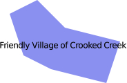
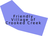
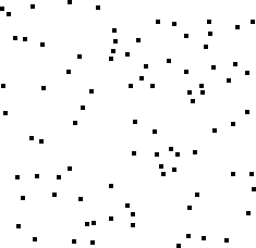
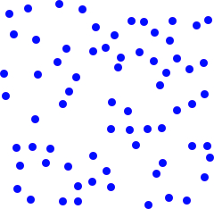
There are two ways in which the TextSymbolizer places text onto the feature being labeled. Using point placement (the default), Mapnik would draw labels on the three features shown previously in the following way:
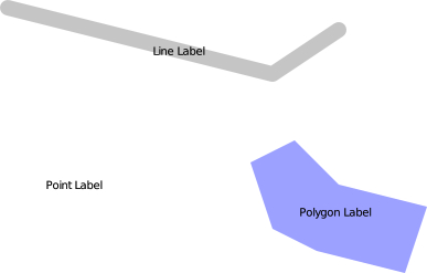
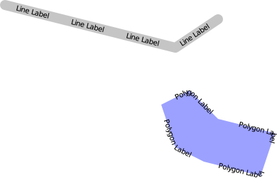
As you can see, the labels are drawn at the center of each feature, and the labels are drawn horizontally with no regard to the orientation of the line. The other option for placing text onto the feature is to use line placement. Labeling the previous features using line placement would result in the following:

Notice that the polygon's label is now drawn along the boundary of the polygon, and the labels now follow the orientation of the line. The point feature isn't labeled at all since the point feature has no lines within it.
You control the placement of the text by setting the symbolizer's label_placement attribute, such as:
sym1.label_placement = mapnik.label_placement.POINT_PLACEMENT
sym2.label_placement = mapnik.label_placement.LINE_PLACEMENT
When labels are placed using LINE_PLACEMENT, Mapnik will by default draw the label once, in the middle of the line. In many cases, however, it makes sense to have the label repeated along the length of the line. To do this, you set the symbolizer's label_spacing attribute, as shown below:
symbolizer.label_spacing = 30
Setting this attribute causes the labels to be repeated along the line or polygon boundary. The value is the amount of space between each repeated label, in pixels. Using the above label spacing, our line and polygon features would be displayed in the following way:
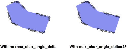
There are several other attributes that can be used to fine-tune the way repeated labels are displayed:
symbolizer.force_odd_labels = True:This tells theTextSymbolizerto always draw an odd number of labels. This can make the labels look better in some situations.symbolizer.max_char_angle_delta = 45:This sets the maximum change in angle (measured in degrees) from one character to the next. Using this can prevent Mapnik from drawing labels around sharp corners. For example:
symbolizer.min_distance = 40:The minimum distance between repeated labels, in pixels.symbolizer.label_position_tolerance = 20:This sets the maximum distance a label can move along the line to avoid other labels and sharp corners. The value is in pixels, and defaults tomin_distance/2.
By default, Mapnik ensures that two labels will never intersect. If possible, it will move the labels to avoid an overlap. If you look closely at the labels drawn around the boundary of the following two polygons, you will see that the position of the left polygon's labels has been adjusted to avoid an overlap:
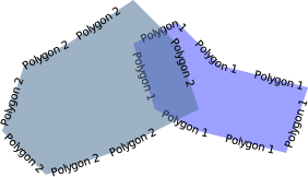
If Mapnik decides that it can't move the label without completely misrepresenting the position of the label then it will hide the label completely. You can see this in the following illustration, where the two polygons are moved so they overlap:
The allow_overlap attribute allows you to change this behaviour:
symbolizer.allow_overlap = True
Instead of hiding the overlapping labels, Mapnik will simply draw them one on top of the other:
The TextSymbolizer will normally draw the text directly onto the map. This works well when the text is placed over a lightly-colored area of the map, but if the underlying area is dark, the text can be hard to read or even invisible:
Of course, you could choose a light text color, but that requires you to know in advance what the background is likely to be. A better solution is to draw a "halo" around the text, as shown in the following image:
The halo_fill and halo_radius attributes allow you to define the color and size of the halo to draw around the text, like this:
symbolizer.halo_fill   = mapnik.Color("white")
symbolizer.halo_radius = 1
The radius is specified in pixels; generally, a small value such as 1 or 2 is enough to ensure that the text is readable against a dark background.
By default, Mapnik calculates the point at which the text should be displayed, and then displays the text centered over that point, as shown here:
You can adjust this positioning in two ways: by changing the vertical alignment, and by specifying a text displacement.
The vertical alignment can be controlled by changing the TextSymbolizer's vertical_alignment attribute. There are three vertical alignment values you can use:
sym2.vertical_alignment = mapnik.vertical_alignment.TOP
sym1.vertical_alignment = mapnik.vertical_alignment.MIDDLE
sym3.vertical_alignment = mapnik.vertical_alignment.BOTTOM
mapnik.vertical_alignment.MIDDLE is the default, and places the label centered vertically over the point, as shown previously.
If you change the vertical alignment to mapnik.vertical_alignment.TOP, the label will be drawn above the point, as shown here:
Conversely, if you change the vertical alignment to mapnik.vertical_alignment.BOTTOM, the label will be drawn below the point:
Your other option for adjusting text positioning is to use the displacement() method to displace the text by a given number of pixels. For example:
symbolizer.displacement(5, 10)
This will shift the label five pixels to the right and ten pixels down from its normal position:
Tip
Beware
Changing the vertical displacement of a label will also change the label's default vertical_alignment value. This can result in your label being moved in unexpected ways because the vertical alignment of the label is changed as a side-effect of setting the vertical displacement. To avoid this, you should always set the vertical_alignment attribute explicitly whenever you change the vertical displacement.
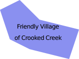
Sometimes a label is too long to be displayed in the way that you might like:
In this case, you can use the wrap_width attribute to force the label to wrap across multiple lines. For example:
symbolizer.wrap_width = 70
This will cause the previous label to be displayed like the following:

The value you specify is the maximum width of each line of text, in pixels.
You can add extra space between each character in a label by setting the character_spacing attribute, like the following:
symbolizer.character_spacing = 3
This results in our polygon being labeled as shown in the following image:
Note
Unfortunately, character spacing only works when the text is drawn using point placement. Line placement is not yet supported.
You can also change the spacing between the various lines using the line_spacing attribute:
symbolizer.line_spacing = 8
Our polygon will then look similar to the following image:
Both the character spacing and the line spacing values are in pixels.
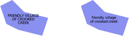
There are times when you might want to change the case of the text being displayed. You can do this by setting the text_convert attribute, as shown by the following:
symbolizer1.text_convert = mapnik.text_convert.toupper
symbolizer2.text_convert = mapnik.text_convert.tolower
These two settings will result in the labels being displayed as follows:
There are two ways of drawing a point using Mapnik: the PointSymbolizer allows you to draw an image at a given point, and the ShieldSymbolizer combines an image with a textual label to produce a "shield".
Let's examine how each of these two symbolizers work.
A PointSymbolizer draws an image at the point. The default constructor takes no arguments and displays each point as a 4x4-pixel black square:
symbolizer = PointSymbolizer()
Alternatively, you can supply the name, type, and dimensions for an image file that the PointSymbolizer will use to draw each point:
symbolizer = PointSymbolizer("point.png", "png", 9, 9)
Tip
Be aware that the PointSymbolizer draws the image centered over the desired point. You may have to add transparent space around the image so that the desired part of the image appears over the desired point. For example, if you wish to draw a pin at an exact position, you might need to format the image as the following:
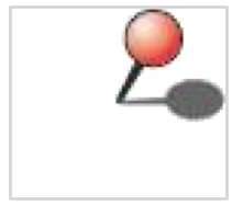
The extra (transparent) whitespace ensures that the point of the pin is in the center of the image, allowing the image to be drawn exactly at the desired position on the map.
Whether you supply an image or not, the PointSymbolizer has two attributes that you can use to modify its behavior:
symbolizer.allow_overlap = True:If you set this attribute to True, all points will be drawn even if the images overlap. The default (False) means that points will only be drawn if they don't overlap.symbolizer.opacity = 0.75:How opaque or transparent to draw the image. A value of0.0will draw the image completely transparent, while a value of1.0(the default) will draw the image completely opaque.
A ShieldSymbolizer draws a textual label and an associated image:
The ShieldSymbolizer works in exactly the same way as having a TextSymbolizer and a PointSymbolizer rendering the same data. The only difference is that the ShieldSymbolizer ensures that the text and image are always displayed together; you'll never get the text without the image, or vice versa.
When you create a ShieldSymbolizer, you have to provide a number of parameters:
symbolizer = mapnik.ShieldSymbolizer(fieldName,
                                     font, fontSize, color,
                                     imageFile, imageFormat,
                                     imageWidth, imageHeight)
Where:
fieldNameis the name of the field or attribute to display as the textual labelfontis the name of the font to use when drawing the textfontSizeof the size of the text, in pointscoloris a Mapnik color object that defines the color to use for drawing the textimageFileis the name (and optional path) of the file that holds the image to displayimageFormatis a string defining the format of the image file (PNG or TIFF)imageWidthis the width of the image file, in pixelsimageHeightis the height of the image file, in pixels
Because ShieldSymbolizer is a subclass of TextSymbolizer, all the positioning and formatting options available for a TextSymbolizer can also be applied to a ShieldSymbolizer. And, because it also draws an image, a ShieldSymbolizer also has the allow_overlap and opacity attributes of a PointSymbolizer.
Be aware that you will most probably need to call the ShieldSymbolizer's displacement() method to position the text correctly as by default the text appears directly over the point, in the middle of the image.
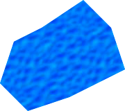
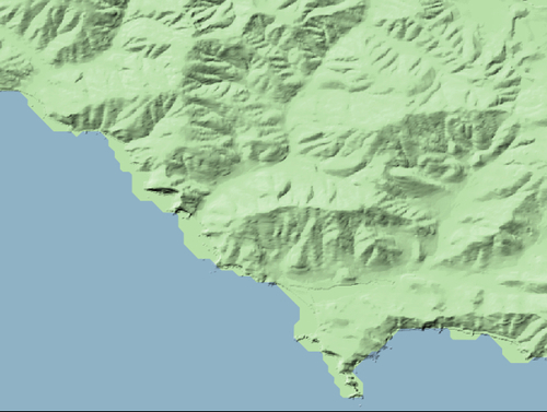
The GDAL and Raster datasources allow you to include raster images within a map. The RasterSymbolizer takes this raster data and displays it within a map layer, as shown in the following image:
Creating a RasterSymbolizer is very simple:
symbolizer = mapnik.RasterSymbolizer()
A RasterSymbolizer will automatically draw the contents of the layer's raster-format datasource onto the map.
The RasterSymbolizer supports the following options for controlling how the raster data is displayed:
symbolizer.opacity = 0.5This controls how opaque the raster image will be. A value of 0.0 makes the image fully transparent, and a value of 1.0 makes it fully opaque. By default, the raster image will be completely opaque.
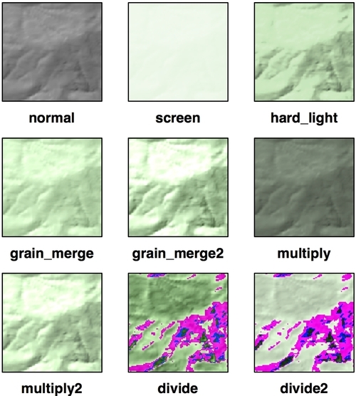
symbolizer.mode = "hard_light"This attribute tells the RasterSymbolizer how to combine the raster data with the previously-rendered map data beneath it. These modes are similar to the way layers are merged in image editing programs such as Photoshop or the GIMP. The following merge modes are supported:
symbolizer.scaling = "fast"This allows you to control the algorithm used to scale the raster image data. The available options are: fast (uses the nearest-neighbor algorithm), bilinear (uses bilinear interpolation across all four color channels), and bilinear8 (uses bilinear interpolation for just a single color channel).
Tip
Mapnik does not currently support on-the-fly reprojection of raster data. If you need to generate a map using a projection that is different from the raster data's projection, you will need to reproject the raster data before it can be displayed, for example by using gdalwarp.
One of the main uses for a RasterSymbolizer is to display a shaded relief background such as the one shown previously. This gives the viewer a good impression of the underlying terrain.
Note
The previous image was created using a Digital Elevation Map (DEM-format) data file taken from the National Elevation Dataset. This file was processed using the gdaldem utility with the hillshade option to create a shaded relief grayscale image. This image was then displayed using a RasterSymbolizer set to hard_light mode, laid on top of a pale green background with the coastline defined from the GSHHS shoreline database. You may find this process useful if you want to display a shaded relief image as a background for your map.
Many of the Mapnik symbolizers require you to supply a color value. These color values are defined using the mapnik.Color class. Instances of mapnik.Color can be created in one of four ways:
mapnik.Color(r, g, b, a)Creates a color object by supplying separate red, green, blue, and alpha (opacity) values. Each of these values should be in the range 0 to 255.
mapnik.Color(r, g, b)Creates a color object by supplying red, green, and blue components. Each value should be in the range 0 to 255. The resulting object will be completely opaque.
mapnik.Color(colorName)Creates a color object by specifying a standard CSS color name. A complete list of the available color names can be found at: http://www.w3.org/TR/css3-color/#svg-color.
mapnik.Color(colorCode)Creates a color object using an HTML color code. For example, #806040 is medium brown.
Once you have set up your datasources, symbolizers, rules, and styles, you can combine them into Mapnik layers and place the various layers together onto a map. To do this, you first create a mapnik.Map object to represent the map as a whole:
map = mapnik.Map(width, height, srs)
You supply the width and height of the map image you want to generate, in pixels, and an optional Proj 4 format initialization string in srs. If you do not specify a spatial reference system, the map will use +proj=latlong +datum=WGS84 (unprojected lat/long coordinates on the WGS84 datum).
After creating the map, you set the map's background color, and add your various styles to the map by calling the map.append_style() method:
map.background = mapnik.Color('white')

map.append_style("countryStyle", countryStyle)
map.append_style("roadStyle", roadStyle)
map.append_style("pointStyle", pointStyle)
map.append_style("rasterStyle", rasterStyle)
...
You also need to create the various layers within the map. To do this, you create a mapnik.Layer object to represent each map layer:
layer = mapnik.Layer(layerName, srs)
Each layer is given a unique name, and can optionally have a spatial reference associated with it. The srs string is a Proj.4 format initialization string; if no spatial reference is given, the layer will use +proj=latlong +datum=WGS84.
Once you have created your map layer, you assign it a datasource and choose the style(s) that will apply to that layer, identifying each style by name:
layer.datasource = myDatasource

layer.styles.append("countryStyle")
layer.styles.append("rasterStyle")
...
Finally, you add your new layer to the map:
map.layers.append(layer)
Let's take a closer look at some of the optional methods and attributes of the Mapnik Map and Layer objects. These can be useful when manipulating map layers, and for setting up rules and layers which selectively apply based on the map's current scale factor.
The mapnik.Map class provides several additional methods and attributes that you may find useful:
map.envelope()This method returns a mapnik.Envelope object representing the area of the map that is to be displayed. The mapnik.Envelope object supports a number of useful methods and attributes, but most importantly includes minx, miny, maxx, and maxy attributes. These define the map's bounding box in map coordinates.
map.aspect_fix_mode = mapnik.aspect_fix.GROW_CANVASThis controls how Mapnik adjusts the map if the aspect ratio of the map's bounds does not match the aspect ratio of the rendered map image. The following values are supported:
GROW_BBOXexpands the map's bounding box to match the aspect ratio of the generated image. This is the default behavior.GROW_CANVASexpands the generated image to match the aspect ratio of the bounding box.SHRINK_BBOXshrinks the map's bounding box to match the aspect ratio of the generated image.SHRINK_CANVASshrinks the generated image to match the aspect ratio of the map's bounding box.ADJUST_BBOX_HEIGHTexpands or shrinks the height of the map's bounding box, while keeping the width constant, to match the aspect ratio of the generated image.ADJUST_BBOX_WIDTHexpands or shrinks the width of the map's bounding box, while keeping the height constant, to match the aspect ratio of the generated image.ADJUST_CANVAS_HEIGHTexpands or shrinks the height of the generated image, while keeping the width constant, to match the aspect ratio of the map's bounding box.ADJUST_CANVAS_WIDTHexpands or shrinks the width of the generated image, while keeping the height constant, to match the aspect ratio of the map's bounding box.
map.scale_denominator()Returns the current scale denominator used to generate the map. The scale denominator depends on the map's bounds and the size of the rendered image.
map.scale()Returns the current scale factor used by the map. The scale factor depends on the map's bounds and the size of the rendered image.
map.zoom_all()Sets the map's bounding box to encompass the bounding box of each of the map's layers. This ensures that all the map data will appear on the map.
map.zoom_to_box(mapnik.Envelope(minX, minY, maxX, maxY))Sets the map's bounding box to the given values. Note that minX, minY, maxX, and maxY are all in the map's coordinate system.
The mapnik.Layer class has the following useful attributes and methods:
layer.envelope()This method returns a mapnik.Envelope object representing the rectangular area of the map that encompasses all the layer's data. The mapnik.Envelope object supports a number of useful methods and attributes, but most importantly includes minx, miny, maxx, and maxy attributes.
layer.active = FalseThis can be used to hide a layer within the map.
layer.minzoom = 1.0/100000This sets the minimum scale factor that must apply if the layer is to appear within the map. If this is not set, the layer will not have a minimum scale factor.
layer.maxzoom = 1.0/10000This sets the maximum scale factor that must apply if the layer is to be drawn onto the map. If this is not set, the layer will not have a maximum scale factor.
layer.visible(1.0/50000)This method returns True if this layer will appear on the map at the given scale factor. The layer is visible if it is active and the given scale factor is between the layer's minimum and maximum values.
After creating your mapnik.Map object and setting up the various symbolizers, rules, styles, datasources, and layers within it, you are finally ready to convert your map into a rendered image.
Before rendering the map image, make sure that you have set the appropriate bounding box for the map so that the map will show the area of the world you are interested in. You can do this by either calling map.zoom_to_box() to explicitly set the map's bounding box to a given set of coordinates, or you can call map.zoom_all() to have the map automatically set its bounds based on the data to be displayed.
Once you have set the bounding box, you can generate your map image by calling the render_to_file() function, as shown below:
mapnik.render_to_file(map, 'map.png')
The parameters are the mapnik.Map object and the name of the image file to write the map to. If you want more control over the format of the image, you can add an extra parameter which defines the image format:
mapnik.render_to_file(map, 'map.png', 'png256')
The supported image formats include:
|
Image Format |
Description |
|---|---|
|
|
A 32-bit PNG format image |
|
|
An 8-bit PNG format image |
|
|
A JPEG-format image |
|
|
An SVG-format image |
|
|
A PDF file |
|
|
A postscript format file |
The render_to_file() function works well when you want to generate a single image from your entire map. Another useful way of rendering maps is to generate a number of "tiles" that can then be stitched together to display the map at a higher resolution:
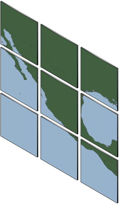
Mapnik provides a helpful function for creating tiles like this out of a single map:
def render_tile_to_file(map, xOffset, yOffset, width, height,
                        fileName, format)
Where:
mapis themapnik.Mapobject containing the map dataxOffsetandyOffsetdefine the top-left corner of the tile, in map coordinateswidthandheightdefine the size of the tile, in map coordinatesfileNameis the name of the file to save the tiled image intoformatis the file format to use for saving this tile
You can simply call this function repeatedly to create the individual tiles for your map. For example:
for x in range(NUM_TILES_ACROSS):
    for y in range(NUM_TILES_DOWN):
        xOffset = TILE_SIZE * x
        yOffset = TILE_SIZE * y
        tileName = "tile_%d_%d.png" % (x, y)
        mapnik.render_tile_to_file(map, xOffset, yOffset,
                                   TILE_SIZE, TILE_SIZE,
                                    tileName, "png")
Another way of rendering a map is to use a Mapnik.Image object to hold the rendered map data in memory. You can then extract the raw image data from the Image object, such as:
image = mapnik.Image(MAP_WIDTH, MAP_HEIGHT)
mapnik.render(map, image)
imageData = image.tostring('png')