
At this stage, we have a complete implementation of the DISTAL system that works as advertized: a user can choose a country, enter a search radius in miles, click on a starting point, and see a high-resolution map showing all the placenames within the desired search radius. We have solved the distance problem, and have all the data needed to search for placenames anywhere in the world.
Of course, we aren't finished yet. There are several areas where our DISTAL application doesn't work as well as it should, including:
- Usability
- Quality
- Performance
- Scalability
Let's take a look at each of these issues, and see how we could improve our design and implementation of the DISTAL system.
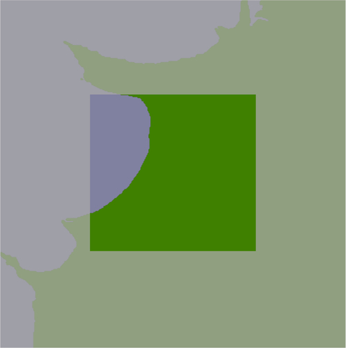
If you explore the DISTAL application, you will soon discover a major usability problem with some of the countries. For example, if you click on the United States in the Select Country page, you will be presented with the following map to click on:

Accurately clicking on a desired point using this map would be almost impossible.
What has gone wrong? The problem here is twofold:
- The United States outline doesn't just cover the mainland US, but also includes the outlying states of Alaska and Hawaii. This increases the size of the map considerably.
- Alaska crosses the 180th meridian—the Alaska Peninsula extends beyond -180° west, and continues across the Aleutian Islands to finish at Attu Island with a longitude of 172° east. Because it crosses the 180th meridian, Alaska appears on both the left and right sides of the world map.
Because of this, the United States map goes from -180° to +180° longitude and +18° to +72° latitude. This map is far too big to be usable.
Even for countries that aren't split into separate outlying states, and which don't cross the 180th meridian, we can't be assured that the maps will be detailed enough to click on accurately. For example, here is the map for Canada:
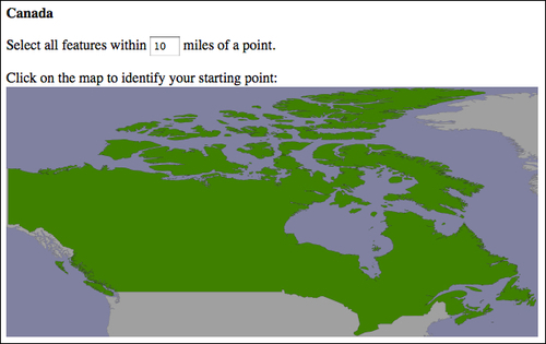
Because Canada is over 3,000 miles wide, accurately selecting a 10-mile search radius by clicking on a point on this map would be an exercise in frustration.
An obvious solution to these usability issues would be to let the user "zoom in" on a desired area of the large-scale map before clicking to select the starting point for the search. Thus, for these larger countries, the user would select the country, choose which portion of the country to search on, and then click on the desired starting point.
This doesn't solve the 180th meridian problem, which is somewhat more difficult. Ideally, you would identify those countries that cross the 180th meridian and reproject them into some other coordinate system that allows their polygons to be drawn contiguously.
As you use the DISTAL system, you will quickly notice some quality issues related to the underlying data that is being used. We are going to consider two such issues: problems with the name data, and problems with the placename lat/long coordinates.
If you look through the list of placenames, you'll notice that some of the names have double parentheses around them, like this:
…
(( Shinavlash ))
(( Pilur ))
(( Kaçarat ))
(( Kaçaj ))
(( Goricë ))
(( Lilaj ))
…
These are names for places that are thought to no longer exist. Also, you will notice that some names have the word historical in them, surrounded by either square brackets or parentheses:
…
Fairbank (historical)
Kopiljača [historical]
Hardyville (historical)
Dorćol (historical)
Sotos Crossing (historical)
Dušanovac (historical)
…
Obviously, these should also be removed. Filtering out the names that should be excluded from the DISTAL database is relatively straightforward, and could be added to our import logic as we read the NationalFile and Geonames files into the database.
Consider the following DISTAL map, covering part of The Netherlands:
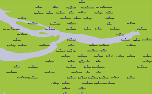
The placement of the cities looks suspiciously regular, as if the cities are neatly stacked into rows and columns. Drawing a grid over this map confirms this suspicion:
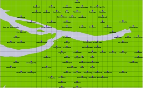
The towns and cities themselves aren't as regularly spaced as this, of course—the problem appears to be caused by inaccurately rounded lat/long coordinates within the international placename data.
This doesn't affect the operation of the DISTAL application, but users may be suspicious about the quality of the results when the placenames are drawn so regularly onto the map. The only solution to this problem would be to find a source of more accurate coordinate data for international placenames.
Our DISTAL application is certainly working, but its performance leaves something to be desired. While the selectCountry.py and selectArea.py scripts run quickly, it can take up to three seconds for showResults.py to complete. Clearly, this isn't good enough: a delay like this is annoying to the user, and would be disastrous for the server as soon as it receives more than 20 requests per minute as it would be receiving more requests than it could process.
Let's take a look at what is going on here. Adding basic timing code to showResults.py reveals where the script is taking most of its time:
Calculating lat/long coordinate took 0.0110 seconds
Identifying placenames took 0.0088 seconds
Generating map took 3.0208 seconds
Building HTML page took 0.0000 seconds
Clearly, the map-generation process is the bottleneck here. Since it only took a fraction of a second to generate a map within the selectArea.py script, there's nothing inherent in the map-generation process that causes this bottleneck. So, what has changed?
It could be that displaying the placenames takes a while, but that's unlikely. It's far more likely to be caused by the amount of map data that we are displaying: the showResults.py script is using high-resolution shoreline outlines taken from the GSHHS dataset rather than the low-resolution country outline taken from the World Borders dataset. To test this theory, we can change the map data being used to generate the map, altering showResults.py to use the low-resolution countries table instead of the high-resolution shorelines table.
The result is a dramatic improvement in speed:
Generating map took 0.1729 seconds
So, how can we make the map generation in showResults.py faster? The answer lies in the nature of the shoreline data and how we are using it. Consider the situation where you are identifying points within 10 miles of Le Havre in France:
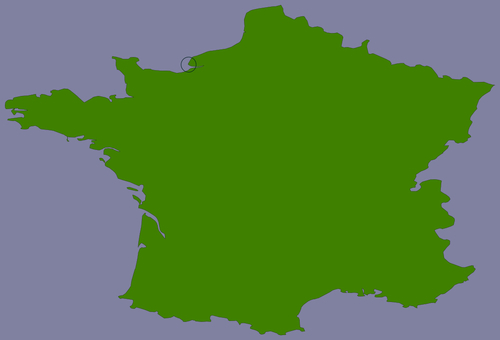
The high-resolution shoreline image would look like this:
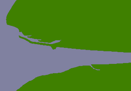
But, this section of coastline is actually part of the following GSHHS shoreline feature:
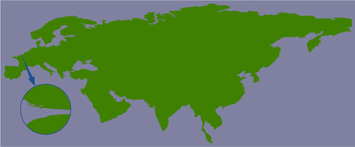
This shoreline polygon is enormous, consisting of over 1.1 million points, and we're only displaying a very small part of it.
Because these shoreline polygons are so big, the map generator needs to read in the entire huge polygon and then discard 99 percent of it to get the desired section of shoreline. Also, because the polygon bounding boxes are so large, many irrelevant polygons are being processed (and then filtered out) when generating the map. This is why showResults.py is so slow.
It is certainly possible to improve the performance of the showResults.py script. Because the DISTAL application only shows points within a certain (relatively small) distance, we can split these enormous polygons into "tiles" that are then pre-calculated and stored in the database.
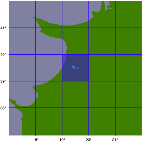
Let's say that we're going to impose a limit of 100 miles to the search radius. We'll also arbitrarily define the tiles to be one whole degree of latitude high, and one whole degree of longitude wide:
Note
Note that we could choose any tile size we like, but have selected whole degrees of longitude and latitude to make it easy to calculate which tile a given lat/long coordinate is inside. Each tile will be given an integer latitude and longitude value, which we'll call iLat and iLong. We can then calculate the tile to use for any given latitude and longitude, like this:
iLat = int(latitude)
iLong = int(longitude)
We can then simply look up the tile with the given iLat and iLong value.
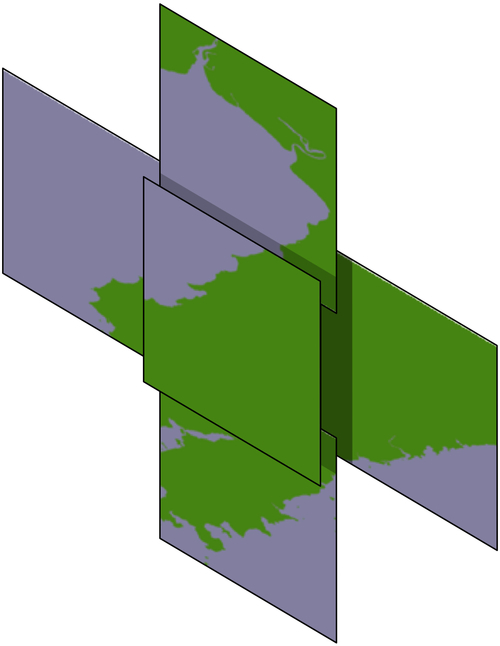
For each tile, we will use the same technique we used earlier to identify the bounding box of the search radius, to define a rectangle 100 miles north, east, west, and south of the tile:
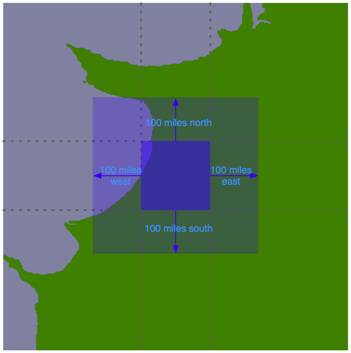
Using the bounding box, we can calculate the intersection of the shoreline data with this bounding box:
Any search done within the tile's boundary, up to a maximum of 100 miles in any direction, will only display shorelines within this bounding box. We simply store this intersected shoreline into the database, along with the lat/long coordinates for the tile, and tell the map generator to use the appropriate tile's outline to display the desired shoreline.
Let's write the code that calculates these tiled shorelines. First off, we'll define a function that calculates the tile bounding boxes. This function, expandRect(), takes a rectangle defined using lat/long coordinates, and expands it in each direction by a given number of meters:
def expandRect(minLat, minLong, maxLat, maxLong, distance):

    geod = pyproj.Geod(ellps="WGS84")
    midLat  = (minLat + maxLat) / 2.0
    midLong = (minLong + maxLong) / 2.0

    try:
        availDistance = geod.inv(midLong, maxLat, midLong,
                                 +90)[2]
        if availDistance >= distance:
            x,y,angle = geod.fwd(midLong, maxLat, 0, distance)
            maxLat = y
        else:
            maxLat = +90
    except:
        maxLat = +90 # Can't expand north.

    try:
        availDistance = geod.inv(maxLong, midLat, +180,
                                 midLat)[2]
        if availDistance >= distance:
            x,y,angle = geod.fwd(maxLong, midLat, 90,
                                 distance)
            maxLong = x
        else:
            maxLong = +180
    except:
        maxLong = +180 # Can't expand east.

    try:
        availDistance = geod.inv(midLong, minLat, midLong,
                                 -90)[2]
        if availDistance >= distance:
            x,y,angle = geod.fwd(midLong, minLat, 180,
                                 distance)
            minLat = y
        else:
            minLat = -90
    except:
        minLat = -90 # Can't expand south.

    try:
        availDistance = geod.inv(maxLong, midLat, -180,
                                 midLat)[2]
        if availDistance >= distance:
            x,y,angle = geod.fwd(minLong, midLat, 270,
                                 distance)
            minLong = x
        else:
            minLong = -180
    except:
        minLong = -180 # Can't expand west.

    return (minLat, minLong, maxLat, maxLong)
Note
Notice that we've added error-checking here, to allow for rectangles close to the North or South Pole.
Using this function, we can calculate the bounding rectangle for a given tile as follows:
minLat,minLong,maxLat,maxLong = expandRect(iLat, iLong,
                                           iLat+1, iLong+1,
                                           MAX_DISTANCE)
We are now ready to load our shoreline polygons into memory:
shorelinePolys = []

cursor.execute("SELECT AsText(outline) FROM shorelines " +
               "WHERE level=1")
for row in cursor:
    outline = shapely.wkt.loads(row[0])
    shorelinePolys.append(outline)
Note
This implementation of the shoreline tiling algorithm uses a lot of memory. If your computer has less than 2 GB of RAM, you may need to store temporary results in the database. Doing this will of course slow down the tiling process, but it will still work.
Then, we create a list-of-lists to hold the shoreline polygons that appear within each tile:
tilePolys = []
for iLat in range(-90, +90):
    tilePolys.append([])
    for iLong in range(-180, +180):
        tilePolys[-1].append([])
For a given iLat/iLong combination, tilePolys[iLat][iLong] will contain a list of the shoreline polygons that appear inside that tile.
We now want to fill the tilePolys array with the portions of the shorelines that will appear within each tile. The obvious way to do this is to calculate the polygon intersections, like this:
shorelineInTile = shoreline.intersection(tileBounds)
Unfortunately, this approach would take a very long time to calculate—just as the map generation takes about 2-3 seconds to calculate the visible portion of a shoreline, it takes about 2-3 seconds to perform this intersection on a huge shoreline polygon. Because there are 360 x 180 = 64,800 tiles, it would take several days to complete this calculation using this naïve approach.
A much faster solution would be to "divide and conquer" the large polygons. We first split the huge shoreline polygon into vertical strips, like this:
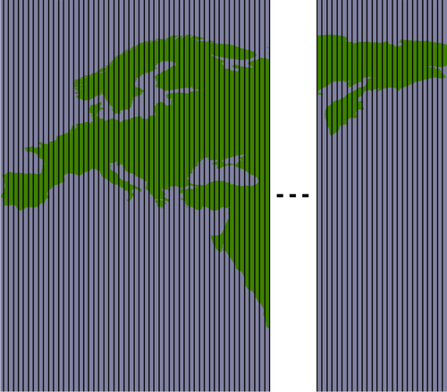
We then split each vertical strip horizontally to give us the individual parts of the polygon that can be merged into the individual tiles:
By dividing the huge polygons into strips, and then further dividing each strip, the intersection process is much faster. Here is the code which performs this intersection; we start by iterating over each shoreline polygon and calculating the polygon's bounds:
for shoreline in shorelinePolys:
    minLong,minLat,maxLong,maxLat = shoreline.bounds
    minLong = int(math.floor(minLong))
    minLat  = int(math.floor(minLat))
    maxLong = int(math.ceil(maxLong))
    maxLat  = int(math.ceil(maxLat))
We then split the polygon into vertical strips:
    vStrips = []
    for iLong in range(minLong, maxLong+1):

        stripMinLat  = minLat
        stripMaxLat  = maxLat
        stripMinLong = iLong
        stripMaxLong = iLong + 1

        bMinLat,bMinLong,bMaxLat,bMaxLong =
                expandRect(stripMinLat, stripMinLong,
                           stripMaxLat, stripMaxLong,
                           MAX_DISTANCE)

        bounds = Polygon([(bMinLong, bMinLat),
                          (bMinLong, bMaxLat),
                          (bMaxLong, bMaxLat),
                          (bMaxLong, bMinLat),
                          (bMinLong, bMinLat)])

        strip = shoreline.intersection(bounds)
        vStrips.append(strip)
Next, we process each vertical strip, splitting the strip into tile-sized blocks and storing it into tilePolys:
    stripNum = 0
    for iLong in range(minLong, maxLong+1):
        vStrip = vStrips[stripNum]
        stripNum = stripNum + 1

        for iLat in range(minLat, maxLat+1):
            bMinLat,bMinLong,bMaxLat,bMaxLong =
                expandRect(iLat, iLong, iLat+1, iLong+1,
                           MAX_DISTANCE)

            bounds = Polygon([(bMinLong, bMinLat),
                              (bMinLong, bMaxLat),
                              (bMaxLong, bMaxLat),
                              (bMaxLong, bMinLat),
                              (bMinLong, bMinLat)])

            polygon = vStrip.intersection(bounds)
            if not polygon.is_empty:
                tilePolys[iLat][iLong].append(polygon)
We're now ready to save the tiled shorelines into the database. Before we do this, we have to create the necessary database table. Using MySQL:
cursor.execute("""
    CREATE TABLE IF NOT EXISTS tiled_shorelines (
        intLat  INTEGER,
        intLong INTEGER,
        outline POLYGON,

        PRIMARY KEY (intLat, intLong))
""")
Using PostGIS:
cursor.execute("DROP TABLE IF EXISTS tiled_shorelines")
cursor.execute("""
    CREATE TABLE tiled_shorelines (
        intLat  INTEGER,
        intLong INTEGER,

        PRIMARY KEY (intLat, intLong))
""")
cursor.execute("""
    SELECT AddGeometryColumn('tiled_shorelines', 'outline',
                             4326, 'POLYGON', 2)
""")
cursor.execute("""
    CREATE INDEX tiledShorelineIndex ON tiled_shorelines
        USING GIST(outline)
""")
And using SpatiaLite:
cursor.execute("DROP TABLE IF EXISTS tiled_shorelines")
cursor.execute("""
    CREATE TABLE tiled_shorelines (
        intLat  INTEGER,
        intLong INTEGER,
        PRIMARY KEY (intLat, intLong))
""")
cursor.execute("""
    SELECT AddGeometryColumn('tiled_shorelines', 'outline',
                             4326, 'POLYGON', 2)
""")
cursor.execute("""
    SELECT CreateSpatialIndex('tiled_shorelines', 'outline')
""")
We can now combine each tile's shoreline polygons into a single MultiPolygon, and save the results into the database:
for iLat in range(-90, +90):
    for iLong in range(-180, +180):
        polygons = tilePolys[iLat][iLong]
        if len(polygons) == 0:
            outline = Polygon()
        else:
            outline = shapely.ops.cascaded_union(polygons)
        wkt = shapely.wkt.dumps(outline)

        cursor.execute("INSERT INTO tiled_shorelines " +
                       "(intLat, intLong, outline) " +
                       "VALUES (%s, %s, GeomFromText(%s))",
                       (iLat, iLong, wkt))
        connection.commit()
All this gives us a new database table, tiled_shorelines, which holds the shoreline data split into partly-overlapping tiles:
Since we can guarantee that all the shoreline data for a given set of search results will be within a single tiled_shoreline record, we can modify showResults.py to use this rather than the raw shoreline data. For PostGIS this is easy; we simply define our datasource dictionary as follows:
iLat  = int(round(startLat))
iLong = int(round(startLong))

sql = "(select outline from tiled_shorelines"
    + " where (iLat=%d) and (iLong=%d)) as shorelines"
    % (iLat, iLong)

datasource = {'type'     : "PostGIS",
              'dbname'   : "distal",
              'table'    : sql,
              'user'     : "...",
              'password' : "..."}
Notice that we're replacing the table name with an SQL sub-selection that directly loads the desired shoreline data from the selected tile.
For SpatiaLite, the code is almost identical:
iLat  = int(round(startLat))
iLong = int(round(startLong))

dbFile = os.path.join(os.path.dirname(__file__),
                      "distal.db")

sql = "(select outline from tiled_shorelines"
    + " where (iLat=%d) and (iLong=%d)) as shorelines"
    % (iLat, iLong)

datasource = {'type'           : "SQLite",
              'file'           : dbFile,
              'table'          : sql,
              'geometry_field' : "outline",
              'key_field'      : "id"}
MySQL is a bit more tricky because we have to use a .VRT file to store the details of the datasource. To do this, we create a temporary file, write the contents of the .VRT file, and then delete the file once we're done:
iLat  = int(round(startLat))
iLong = int(round(startLong))

fd,filename = tempfile.mkstemp(".vrt",
                               dir=os.path.dirname(__file__))
os.close(fd)

vrtFile = os.path.join(os.path.dirname(__file__),
                       filename)

f = file(vrtFile, "w")
f.write('<OGRVRTDataSource>
')
f.write('  <OGRVRTLayer name="shorelines">
')
f.write('    <SrcDataSource>MYSQL:distal,user=USER,' +
             'pass=PASS,tables=tiled_shorelines' +
             '</SrcDataSource>
')
f.write('    <SrcSQL>
')
f.write('      SELECT outline FROM tiled_shorelines WHERE ' +
              '(intLat=%d) AND (intLong=%d)
' % (iLat, iLong)
f.write('    </SrcSQL>
')
f.write('  </OGRVRTLayer>
')
f.write('</OGRVRTDataSource>')
f.close()

datasource = {'type'  : "OGR",
              'file'  : vrtFile,
              'layer' : "shorelines"}

imgFile = mapGenerator.generateMap(...)

os.remove(vrtFile)
With these changes in place, the showResults.py script will use the tiled shorelines rather than the full shoreline data downloaded from GSHHS. Let's now take a look at how much of a performance improvement these tiled shorelines give us.
As soon as you run this new version of the DISTAL application, you'll notice a huge improvement in speed: showResults.py now seems to return its results almost instantly. Where before the map generator was taking 2-3 seconds to generate the high-resolution maps, it's now only taking a fraction of a second:
Generating map took 0.1705 seconds
That's a dramatic improvement in performance: the map generator is now 15-20 times faster than it was, and the total time taken by the showResults.py script is now less than a quarter of a second. That's not bad for a relatively simple change to our underlying map data!
If changing the way the underlying map data is structured made such a difference to the performance of the system, you might wonder what other performance improvements could be made. In general, improving performance is all about making your code more efficient (removing bottlenecks), and reducing the amount of work that your code has to do (precalculating and caching data).
There aren't any real bottlenecks in our DISTAL CGI scripts. All the data is static, and we don't have any complex loops in our scripts that could be optimized. There is, however, one further operation that could possibly benefit from precalculations: the process of identifying all placenames in a given area.
At present, our entire database of placenames is being checked for each search query. Of course, we're using a spatial index, which makes this process fast, but we could in theory eke some more performance gains out of our code by grouping placenames into tiles, just as we did with the shoreline data, and then only checking those placenames that are in the current tile rather than the entire database of several million placenames.
Before we go down this route, though, we need to do a reality check: is it really worth implementing this optimization? If you look back at the timing results earlier in this chapter, you'll see that the placename identification is already very fast:
Identifying placenames took 0.0088 seconds
Even if we were to group placenames by tile and limit the placename searching to just one tile, it's unlikely that we'd improve the time taken. In fact, it could easily get worse. Remember:
"Premature Optimization is the Root of All Evil." - Donald Knuth.
Note
Geo-spatial applications often make use of a caching tile server to avoid unnecessarily rendering the same maps over and over. This isn't suitable for the DISTAL application; because the user clicks on a point to identify the search circle, the generated map will be different each time, and there is no real possibility of caching and re-using the rendered maps. We will look at caching tile servers in Chapter 9, Web Frameworks for Python Geo-Spatial Development as they are very useful for other types of geo-spatial applications.
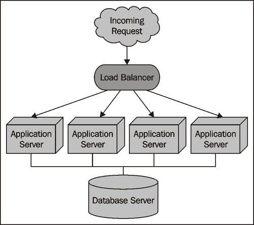
Reducing the processing time from 3.0 to 0.2 seconds means that your application could handle up to 250 requests per minute instead of 20 requests per minute. But, what if you wanted to make DISTAL available on the Internet and had to support up to 25,000 requests per minute? Obviously, improving performance won't be enough, no matter how much you optimize your code.
Allowing the system to scale like this involves running the same software across multiple servers, and using a load balancer to share the incoming requests among the various servers:
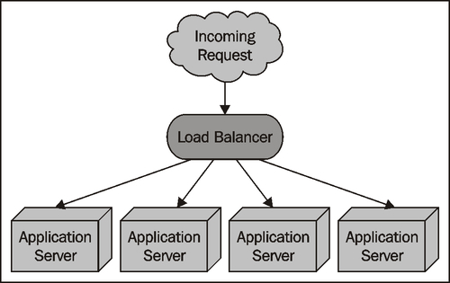
Fortunately, the DISTAL application is ideally suited to using a load balancer in this way: the application has no need to save the user's state in the database (everything is passed from one script to the next using CGI parameters), and the database itself is read-only. This means it would be trivial to install the DISTAL CGI scripts and the fully-populated database onto several servers, and use load balancing software such as nginx (http://nginx.org/en) to share incoming requests among these servers.
Of course, not all geo-spatial applications will be as easy to scale as DISTAL. A more complicated application is likely to need to store user state, and will require read/write access rather than just read-only access to the database. Scaling these types of systems is a challenge.
If your application involves intensive processing of geo-spatial data, you may be able to have a dedicated database server shared by multiple application servers:
As long as the database server is able to serve the incoming requests fast enough, your application servers can do the heavy processing work in parallel. This type of architecture can support a large number of requests—provided the database is able to keep up.
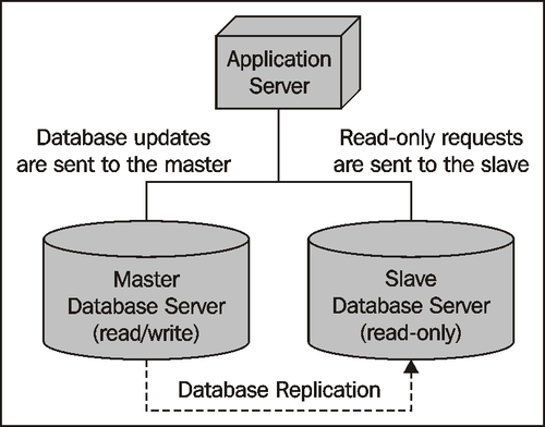
If you reach the stage where a single database server can't manage all the requests, you can redesign your system to use database replication. The most straightforward way to do this is to have one database that accepts changes to the data (the "master"), and a read-only copy of the database (the "slave") that can process requests, but can't make updates. You then set up master-slave database replication so that any changes made to the master database get replicated automatically to the slave. Finally, you need to change your application so that any requests that alter the database get sent to the master, and all other requests get sent to the slave:
Of course, if your application needs to scale to support huge volumes, you may end up with multiple slaves, and use an internal database load balancer to share the read-only requests among the available slaves:
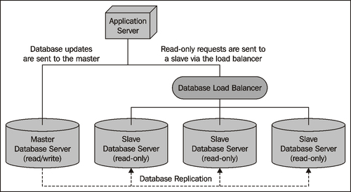
There are other solutions, such as having multiple masters and memory-based database clusters for high-speed retrieval, but these are the main ways in which you can scale your geo-spatial applications.
Note
Database replication is one of the few areas where MySQL outshines PostGIS for geo-spatial development. PostGIS (via its underlying PostgreSQL database engine) currently does not support database replication out of the box; there are third-party tools available that implement replication, but they are complex and difficult to set up. MySQL, on the other hand, supports replication from the outset, and is very easy to set up. There have been situations where geo-spatial developers have abandoned PostGIS in favor of MySQL simply because of its built-in support for database replication.